Posted on 

Forward and backward propagation in neural networks

Deduce forward propagation and back propagation algorithms of neural network with single hidden layer, and program (neural network in ‘Sklearn’ can be used).

  • discuss the impact of 10,30,100,300,1000, different number of hidden nodes on network performance.

  • Explore the influence of different learning rate and iteration times on network performance.

  • Change the standardized method of data to explore the impact on training.
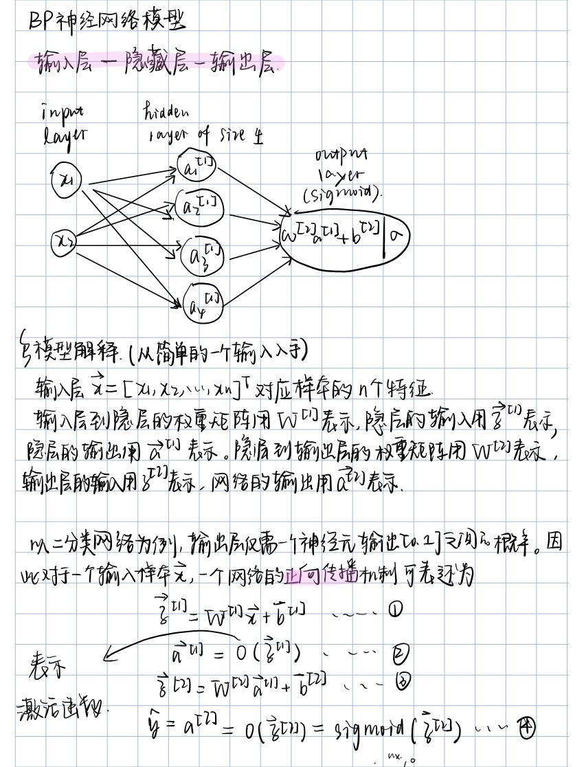
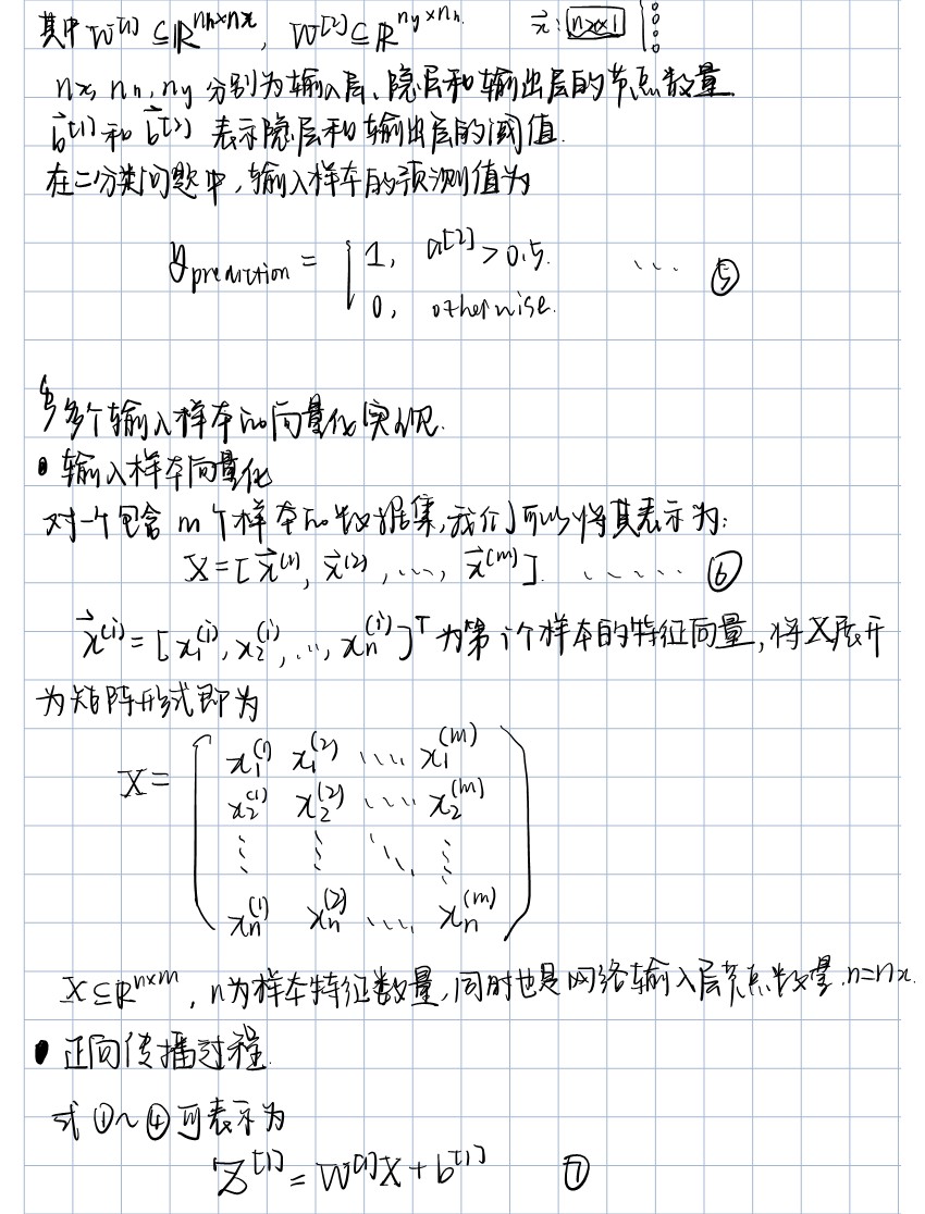
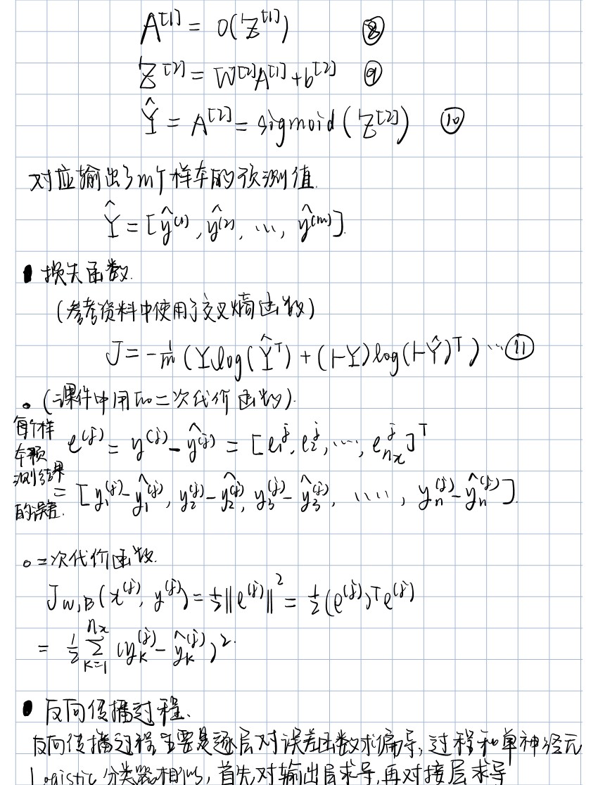
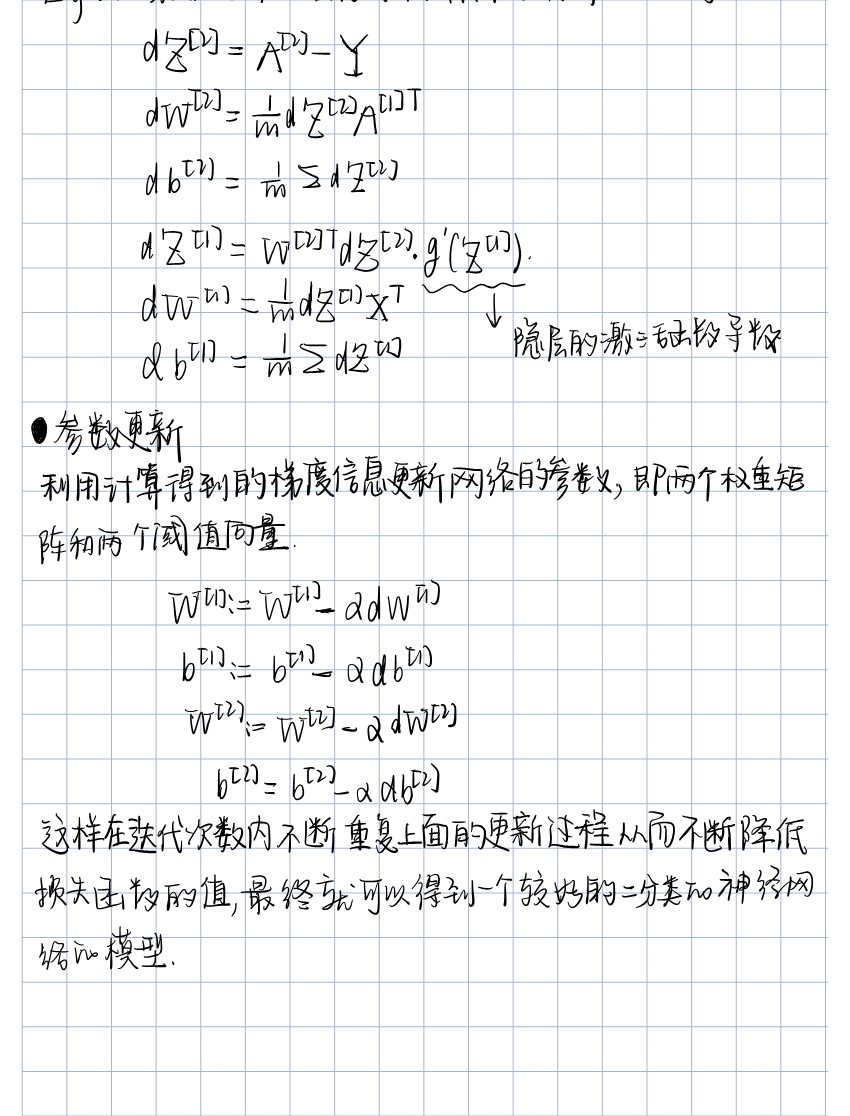
Derivation


Code

Load data

# 1、载入数据
import numpy as np
import tensorflow as tf
import tensorflow.examples.tutorials.mnist.input_data as input_data

# 读取mnist数据
mnist = input_data.read_data_sets('MNIST_data/', one_hot=True)

Construct network

# 2.建立模型

# 2.1 构建输入层
x = tf.placeholder(tf.float32, [None, 784], name='X')
y = tf.placeholder(tf.float32, [None, 10], name='Y')

# 2.2 构建隐藏层
# 隐藏层神经元数量(随意设置)
H1_NN = 256
# 权重
W1 = tf.Variable(tf.random_normal([784, H1_NN]))
# 偏置项
b1 = tf.Variable(tf.zeros([H1_NN]))

Y1 = tf.nn.relu(tf.matmul(x, W1) + b1)

# 2.3 构建输出层
W2 = tf.Variable(tf.random_normal([H1_NN, 10]))
b2 = tf.Variable(tf.zeros([10]))

forward = tf.matmul(Y1, W2) + b2
pred = tf.nn.softmax(forward)

Train the model

# 3.训练模型

# 3.1 定义损失函数
# tensorflow提供了下面的函数,用于避免log(0)值为Nan造成数据不稳定
loss_function = tf.reduce_mean(tf.nn.softmax_cross_entropy_with_logits(logits=forward, labels=y))
# # 交叉熵损失函数
# loss_function = tf.reduce_mean(-tf.reduce_sum(y*tf.log(pred), reduction_indices=1))

# 3.2 设置训练参数
train_epochs = 40 # 训练轮数
batch_size = 50 # 单次训练样本数(批次大小)
# 一轮训练的批次数
total_batch = int(mnist.train.num_examples / batch_size)
display_step = 1 # 显示粒数
learning_rate = 0.01 # 学习率

# 3.2 选择优化器
optimizer = tf.train.AdamOptimizer(learning_rate).minimize(loss_function)

# 3.3定义准确率
correct_prediction = tf.equal(tf.argmax(y, 1), tf.argmax(pred, 1))
accuracy = tf.reduce_mean(tf.cast(correct_prediction, tf.float32))

# 3.4 模型的训练
# 记录训练开始的时间
from time import time

startTime = time()

sess = tf.Session()
sess.run(tf.global_variables_initializer())

for epoch in range(train_epochs):
for batch in range(total_batch):
# 读取批次训练数据
xs, ys = mnist.train.next_batch(batch_size)
# 执行批次训练
sess.run(optimizer, feed_dict={x: xs, y: ys})
# 在total_batch批次数据训练完成后,使用验证数据计算误差和准确率,验证集不分批
loss, acc = sess.run([loss_function, accuracy], feed_dict={x: mnist.validation.images, y: mnist.validation.labels})
# 打印训练过程中的详细信息
if (epoch + 1) % display_step == 0:
print('训练轮次:', '%02d' % (epoch + 1),
'损失:', '{:.9f}'.format(loss),
'准确率:', '{:.4f}'.format(acc))
print('训练结束')
# 显示总运行时间
duration = time() - startTime
print("总运行时间为:", "{:.2f}".format(duration))

Evaluation

# 4.评估模型
accu_test = sess.run(accuracy,
feed_dict={x: mnist.test.images, y: mnist.test.labels})
print('测试集准确率:', accu_test)

Application

# 5.应用模型
prediction_result = sess.run(tf.argmax(pred, 1), feed_dict={x: mnist.test.images})
# 查看预测结果的前10项
print("前10项的结果:", prediction_result[0:10])

# 5.1找出预测错误的样本
compare_lists = prediction_result == np.argmax(mnist.test.labels, 1)
print(compare_lists)
err_lists = [i for i in range(len(compare_lists)) if compare_lists[i] == False]
print('预测错误的图片:', err_lists)
print('预测错误图片的总数:', len(err_lists))

# 定义一个输出错误分类的函数
import numpy as np


def print_predict_errs(labels, # 标签列表
prediction): # 预测值列表
count = 0
compare_lists = (prediction == np.argmax(labels, 1))
err_lists = [i for i in range(len(compare_lists)) if compare_lists[i] == False]
for x in err_lists:
print('index=' + str(x) + '标签值=', np.argmax(labels[x]), '预测值=', prediction[x])
count = count + 1
print("总计:" + str(count))


print_predict_errs(labels=mnist.test.labels, prediction=prediction_result)

# 可视化
import matplotlib.pyplot as plt


def plot_images_labels_prediction(images, # 图像列表
labels, # 标签列表
predication, # 预测值列表
index, # 从第index个开始显示
num=10): # 缺省一次显示10幅
fig = plt.gcf() # 获取当前图表,get current figure
fig.set_size_inches(10, 12) # 设为英寸,1英寸=2.53厘米
if num > 25:
num = 25 # 最多显示25个子图
for i in range(0, num):
ax = plt.subplot(5, 5, i + 1) # 获取当前要处理的子图
# 显示第index图像
ax.imshow(np.reshape(images[index], (28, 28)), cmap='binary')

# 构建该图上显示的title
title = 'label=' + str(np.argmax(labels[index]))
if len(predication) > 0:
title += ",predict=" + str(predication[index])

# 显示图上的title信息
ax.set_title(title, fontsize=10)
ax.set_xticks([]) # 不显示坐标轴
ax.set_yticks([])
index += 1

plt.show()


plot_images_labels_prediction(mnist.test.images,
mnist.test.labels,
prediction_result, 10, 25)
plot_images_labels_prediction(mnist.test.images,
mnist.test.labels,
prediction_result, 610, 20)

Result

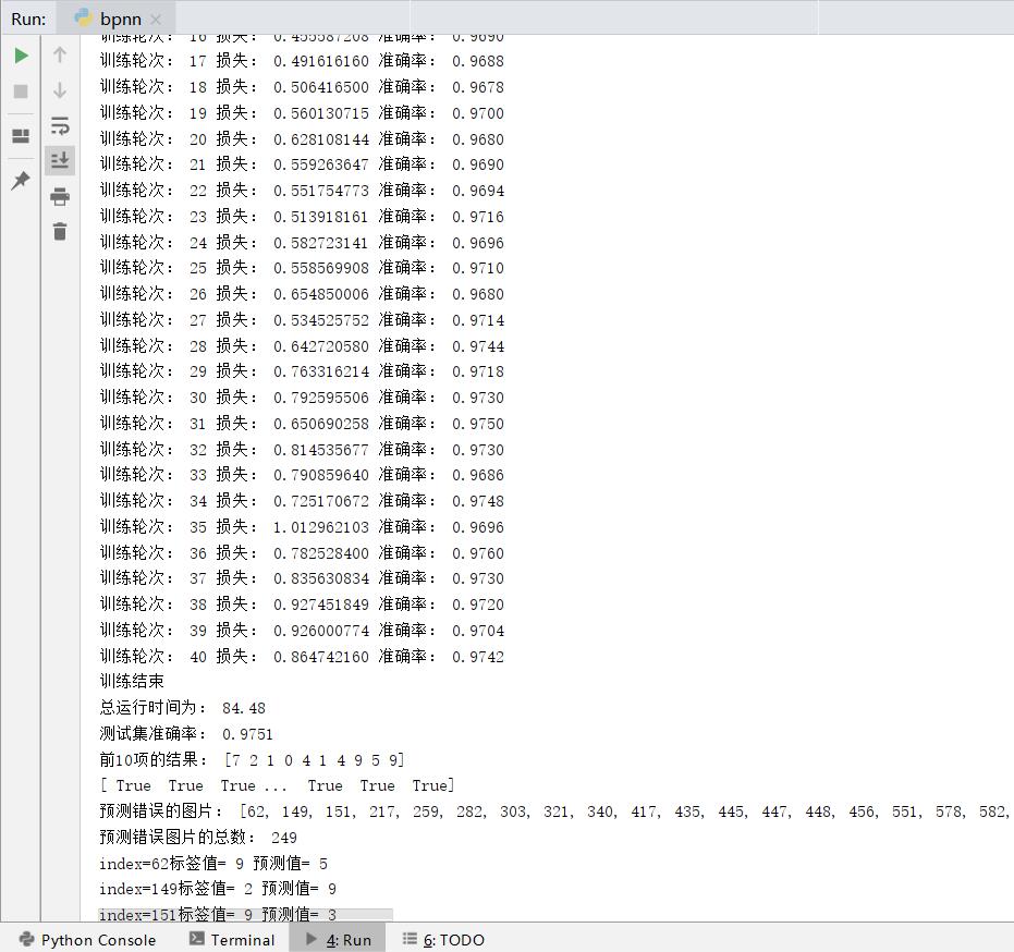
The number of hidden layer nodes: 256
Learning Rate: 0.01
Epochs: 40

Optimization

The number of hidden layer nodes

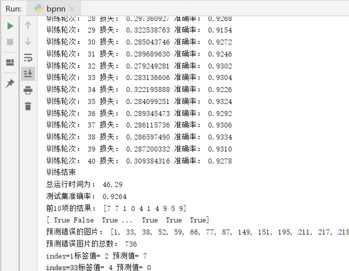
The number of hidden layer nodes: 10

# of hidden layer nodes Running Time/s False Acc.
10 46.29 736 0.9264
30 43.46 528 0.9472
100 59.06 343 0.9657
256 84.48 249 0.9751
300 76.64 269 0.9731
1000 302.27 240 0.976

As can be seen from the table, the accuracy increases with the increase of the number of hidden layer nodes, and the increase rate gradually decreases.

Learning Rate

LR Running Time/s False Acc.
0.005 78.81 231 0.9769
0.01 84.48 249 0.9751
0.02 69.72 446 0.9554
0.1 73.87 2561 0.7439

As can be seen from the table, the accuracy decreases with the increase of the learning rate. When the learning rate is lower than 0.01, the rate of improvement of image classification accuracy is small.

Epochs

Epochs Running Time/s False Acc.
20 37.12 307 0.9693
40 84.48 249 0.9751
100 184.39 239 0.9761

As can be seen from the table, the number of iterations has a great impact on the total running time, and the accuracy increases with the increase of the number of iterations, but the number of nodes in the hidden layer and the learning rate are the decisive factors for the accuracy.

Implement a one-layer network

def layer_sizes(X, Y):
n_x = X.shape[0] # size of input layer
n_h = 4 # size of hidden layer
n_y = Y.shape[0] # size of output layer
return (n_x, n_h, n_y)
def initialize_parameters(n_x, n_h, n_y):
W1 = np.random.randn(n_h, n_x)*0.01
b1 = np.zeros((n_h, 1))
W2 = np.random.randn(n_y, n_h)*0.01
b2 = np.zeros((n_y, 1))

assert (W1.shape == (n_h, n_x))
assert (b1.shape == (n_h, 1))
assert (W2.shape == (n_y, n_h))
assert (b2.shape == (n_y, 1))
parameters = {"W1": W1,
"b1": b1,
"W2": W2,
"b2": b2}

return parameters
def forward_propagation(X, parameters):
# Retrieve each parameter from the dictionary "parameters"
W1 = parameters['W1']
b1 = parameters['b1']
W2 = parameters['W2']
b2 = parameters['b2']
# Implement Forward Propagation to calculate A2 (probabilities)
Z1 = np.dot(W1, X) + b1
A1 = np.tanh(Z1)
Z2 = np.dot(W2, Z1) + b2
A2 = sigmoid(Z2)
assert(A2.shape == (1, X.shape[1]))
cache = {"Z1": Z1,
"A1": A1,
"Z2": Z2,
"A2": A2}
return A2, cache
def compute_cost(A2, Y, parameters):
m = Y.shape[1] # number of example
# Compute the cross-entropy cost
logprobs = np.multiply(np.log(A2),Y) + np.multiply(np.log(1-A2), 1-Y)
cost = -1/m * np.sum(logprobs)
cost = np.squeeze(cost) # makes sure cost is the dimension we expect.
assert(isinstance(cost, float))
return cost
def backward_propagation(parameters, cache, X, Y):
m = X.shape[1]
# First, retrieve W1 and W2 from the dictionary "parameters".
W1 = parameters['W1']
W2 = parameters['W2']
# Retrieve also A1 and A2 from dictionary "cache".
A1 = cache['A1']
A2 = cache['A2']
# Backward propagation: calculate dW1, db1, dW2, db2.
dZ2 = A2-Y
dW2 = 1/m * np.dot(dZ2, A1.T)
db2 = 1/m * np.sum(dZ2, axis=1, keepdims=True)
dZ1 = np.dot(W2.T, dZ2)*(1-np.power(A1, 2))
dW1 = 1/m * np.dot(dZ1, X.T)
db1 = 1/m * np.sum(dZ1, axis=1, keepdims=True)
grads = {"dW1": dW1,
"db1": db1,
"dW2": dW2,
"db2": db2}
return grads
def update_parameters(parameters, grads, learning_rate = 1.2):
# Retrieve each parameter from the dictionary "parameters"
W1 = parameters['W1']
b1 = parameters['b1']
W2 = parameters['W2']
b2 = parameters['b2']
# Retrieve each gradient from the dictionary "grads"
dW1 = grads['dW1']
db1 = grads['db1']
dW2 = grads['dW2']
db2 = grads['db2']
# Update rule for each parameter
W1 -= dW1 * learning_rate
b1 -= db1 * learning_rate
W2 -= dW2 * learning_rate
b2 -= db2 * learning_rate
parameters = {"W1": W1,
"b1": b1,
"W2": W2,
"b2": b2}
return parameters
def nn_model(X, Y, n_h, num_iterations = 10000, print_cost=False):
np.random.seed(3)
n_x = layer_sizes(X, Y)[0]
n_y = layer_sizes(X, Y)[2]
# Initialize parameters, then retrieve W1, b1, W2, b2. Inputs: "n_x, n_h, n_y". Outputs = "W1, b1, W2, b2, parameters".
parameters = initialize_parameters(n_x, n_h, n_y)
W1 = parameters['W1']
b1 = parameters['b1']
W2 = parameters['W2']
b2 = parameters['b2']
# Loop (gradient descent)
for i in range(0, num_iterations):
# Forward propagation. Inputs: "X, parameters". Outputs: "A2, cache".
A2, cache = forward_propagation(X, parameters)
# Cost function. Inputs: "A2, Y, parameters". Outputs: "cost".
cost = compute_cost(A2, Y, parameters)
# Backpropagation. Inputs: "parameters, cache, X, Y". Outputs: "grads".
grads = backward_propagation(parameters, cache, X, Y)
# Gradient descent parameter update. Inputs: "parameters, grads". Outputs: "parameters".
parameters = update_parameters(parameters, grads, learning_rate=1.2)
# Print the cost every 1000 iterations
if print_cost and i % 1000 == 0:
print ("Cost after iteration %i: %f" %(i, cost))

return parameters