Sentiment Analysis | Netizen Sentiment Recognition During COVID-19

The emergence of the COVID-19 has disrupted our normal life. People’s psychological state can also receive a great negative impact. We chose such a topic with humanistic concern in Data Warehouse and Data Mining course, hoping that through Weibo posts we can gain more insight into people’s emotional state during the COVID-19. We are awarded the best project (1/23) in this course, and we think we could do more in psychological care during COVID-19.

Data Source and Data Structure

This data comes from a data mining competition organized by DataFountain. The data set is a collection of Weibo crawled during the COVID-19. The link to the dataset is here.

The dataset cannot be downloaded directly from the official website because the competition has ended, the dataset can also be found on Kaggle.

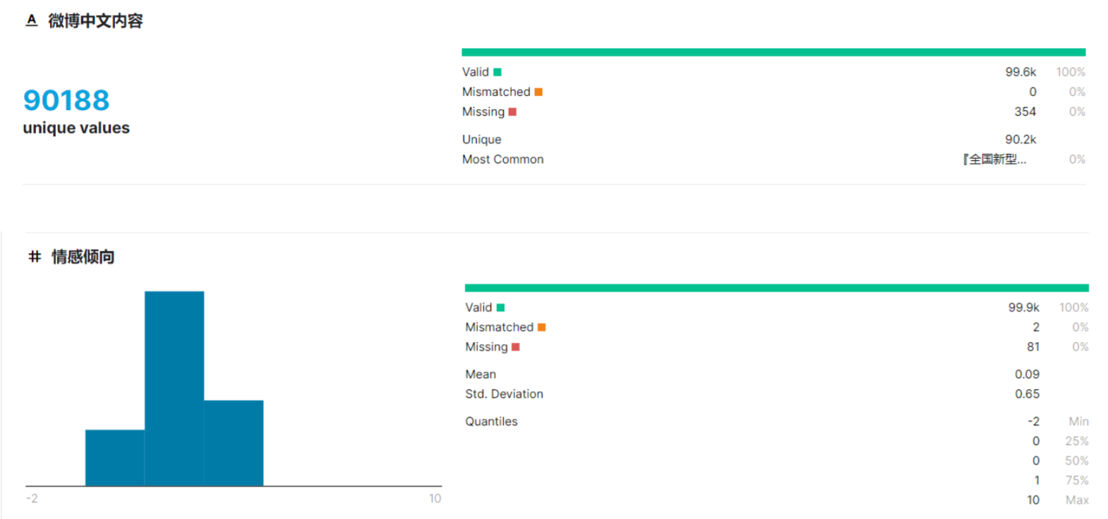
We used 100,000 posts from the training set provided by the competition website, but considering the time and computational cost, I only used the first 10,000 posts with annotations, and divided them into a training set and a test set in a 7/3 ratio. This dataset was based on 230 keywords related to the topic of “新冠肺炎”, which means COVID-19 in Chinese.

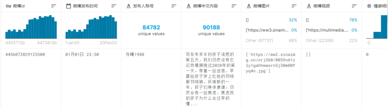
1,000,000 Weibo posts were collected from January 1, 2020 to February 20, 2020, and 100,000 Weibo posts were labeled with three categories: 1 (positive), 0 (neutral) and -1 (negative). The data is stored in csv format in nCoV-100k.labeled.csv file. The original dataset contains 100,000 user-labeled posts in the following format: [post id, posting time, posting account, content, photos, videos, sentiment].

The original dataset has six attributes: post id (hashcode), posting time (Date), posting account (String), content (String), photos (String), and videos (String). Predicting sentiment(Int) by the above attributes. The purpose of this project is to use word bag preprocessing, TF-IDF preprocessing, word2vec and compare their effects, focusing on text processing and text sentiment analysis. So we only chose content attribute to predict the sentiment. (It was hard for us to read the emotion from photos and videos.)

Here is the statistical information of the dataset from Kaggle.

The bar chart shows that the number of positive, neutral and negative posts varies considerably, with the highest number of neutral posts.

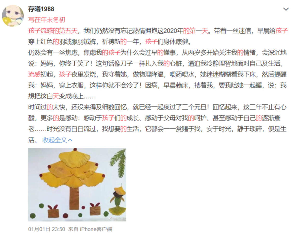
Here is the first post in dataset.

We found this posts in Weibo APP.

Data Preprocessing

We Used Kaggle Kernel. Kaggle provides free access to the Nvidia K80 GPU in the kernel. This benchmark shows that using the GPU for your kernel can achieve a 12.5x speedup in the training of deep learning models.

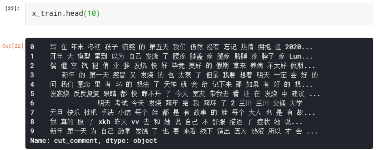
Data import and turncut

import pandas as pd filepath = '/kaggle/input/chinese-text-multi-classification/nCoV_100k_train.labled.cs v' file_data = pd.read_csv(filepath)
data = file_data.head(10000)
# chose content and sentiment
data = data[['微博中⽂内容', '情感倾向']]

Handling missing values

# handling missing values
data.isnull().sum()
data = data.dropna()

Remove meaningless symbols

import re 

def clean_zh_text(text): 
    # keep English, digital and Chinese 
    comp = re.compile('[^A-Z^a-z^0-9^\u4e00-\u9fa5]')
    return comp.sub('', text)
data['微博中⽂内容'] = data.微博中⽂内容.apply(clean_zh_text)

Word Cut

# word cut 
import jieba 
def chinese_word_cut(mytext): 
    return " ".join(jieba.cut(mytext))

data['cut_comment'] = data.微博中⽂内容.apply(chinese_word_cut)

# divided them into a training set and a test set in a 7/3 ratio.
lentrain = int((10000-30)*0.7) 
lentest = int((10000-30)*0.3) 
x_train = data.head(lentrain)['微博中⽂内容'] 
y_train = data.head(lentrain)['情感倾向'] 
x_test = data.tail(lentest)['微博中⽂内容']
y_test = data.tail(lentest)['情感倾向']

Import Stop Words

# import stop words
stpwrdpath = "/kaggle/input/stop-wordstxt/stop_words.txt" 
stpwrd_dic = open(stpwrdpath, 'rb') 
stpwrd_content = stpwrd_dic.read() 

#transform into list 
stpwrdlst = stpwrd_content.splitlines()
stpwrd_dic.close()

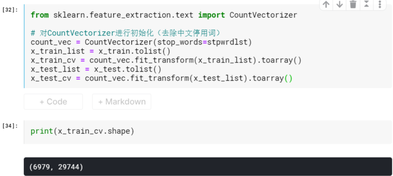
Word Bag Preprocess

from sklearn.feature_extraction.text 
import CountVectorizer

# CountVectorizer initialize
count_vec = CountVectorizer(stop_words=stpwrdlst) 
x_train_list = x_train.tolist() 
x_train_cv = count_vec.fit_transform(x_train_list).toarray() 
x_test_list = x_test.tolist()
x_test_cv = count_vec.fit_transform(x_test_list).toarray()

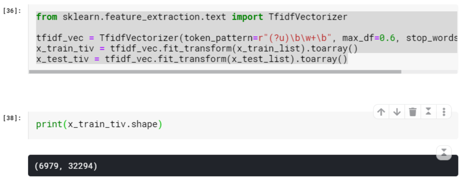
TF-IDF Preprocess

from sklearn.feature_extraction.text import TfidfVectorizer 
tfidf_vec = TfidfVectorizer(token_pattern=r"(?u)\b\w+\b", max_df=0.6, stop_words=stpwr dlst) 
x_train_tiv = tfidf_vec.fit_transform(x_train_list).toarray()
x_test_tiv = tfidf_vec.fit_transform(x_test_list).toarray()

word2vec embedding

# word2vec 
from gensim.models import Word2Vec 
model = Word2Vec(x_train_list, hs=1,min_count=1,window=10,size=100)
from gensim.test.utils import common_texts, get_tmpfile 
path = get_tmpfile("word2vec.model") 
model.save("word2vec.model")
# model = Word2Vec.load("word2vec.model")

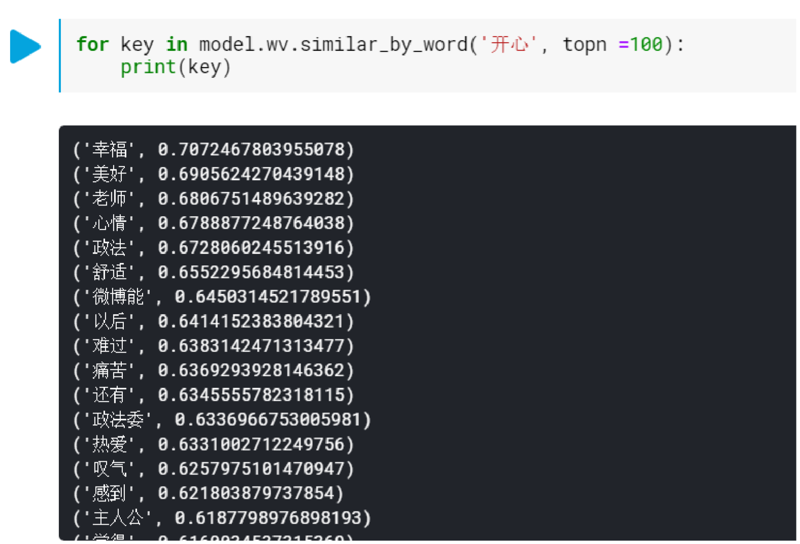
The corpus of 10,000 training data is still a bit small, but the results are slightly more productive. For example, if we look at the close synonyms of “开心”(happy), we can see that the results returned are more positive.

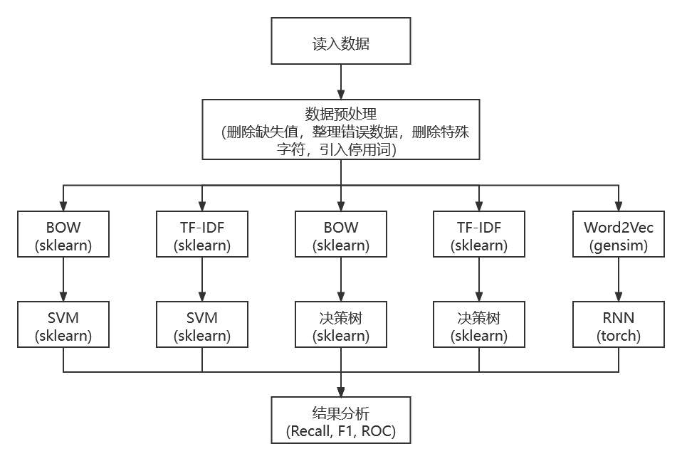
Data Mining Algorithm

In this section, we will use SVM, decision tree and RNN algorithms to achieve classification. The embedding obtained by BOW and TF-IDF will be classified by SVM and decision tree algorithms, respectively, while the embedding obtained by Word2Vec will be classified by RNN.

The embedding obtained from Word2Vec will be classified using RNN. The detailed algorithm flow is as follows.

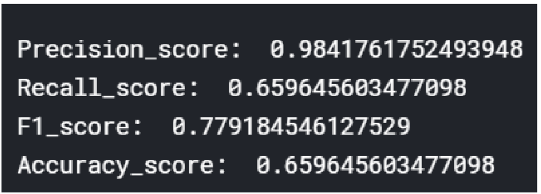
BOW + SVM

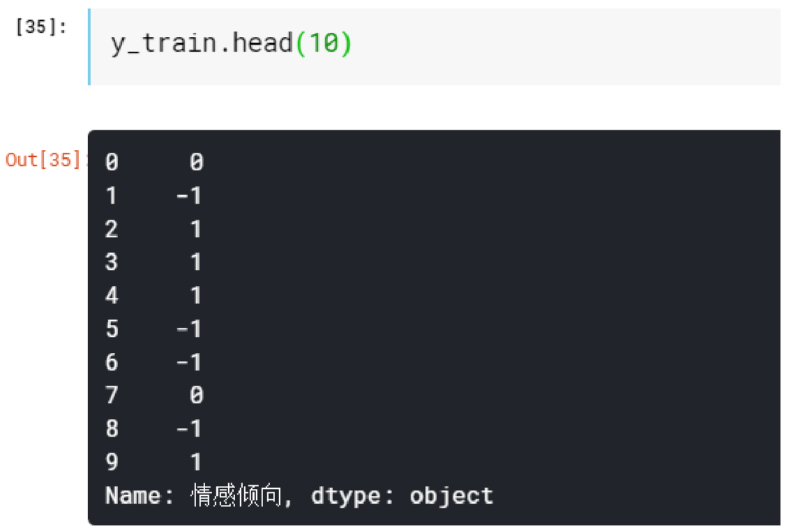
The 35596-dimensional embedding of the Weibo posts obtained by BOW is used as the input of the SVM in the sklearn package.
The parameters are as follows.

clf = svm.SVC(C=0.8, kernel='rbf', gamma=20, decision_function_shape='ovr')

from sklearn.preprocessing import StandardScaler 
scale = StandardScaler() 
scale_fit = scale.fit(x_cv) 
#x = scale_fit.transform(x) 
lentrain = int((10000-30)*0.7) 
lentest = int((10000-30)*0.3)

x_train_cv = scale_fit.transform(x_cv[:lentrain]) 
y_train = y[:lentrain] 
x_test_cv = scale_fit.transform(x_cv[(-1)*lentest-1:-1]) 
y_test = y[(-1)*lentest-1:-1] 
print(x_train_cv.shape) 
print(y_train.shape) 
print(x_test_cv.shape)
print(y_test.shape)

TIPS:

• SVM and Decision Tree algorithms for 10,000 of 30,000-dimensional data can take a lot of time, and sklearn does not support GPU computing.
• When you encounter a very large dataset, you should first use a small demo to check the correctness of the code, and then run a large demo with a large amount of data.
• BOW and TF-IDF should be used first before dividing the test and training sets, otherwise the test and training sets will not have the same dimensionality! It took a lot of time to fix this error.
• Due to the excessive number of dimensions, remember to normalize the data before SVM.

# prepare the data
from sklearn.preprocessing import StandardScaler
scale = StandardScaler()
scale_fit = scale.fit(x_cv)
#x = scale_fit.transform(x)
lentrain = int((10000-30)*0.7)
lentest = int((10000-30)*0.3)

x_train_cv = scale_fit.transform(x_cv[:lentrain])
y_train = y[:lentrain]
x_test_cv = scale_fit.transform(x_cv[(-1)*lentest-1:-1])
y_test = y[(-1)*lentest-1:-1]
print(x_train_cv.shape)
print(y_train.shape)
print(x_test_cv.shape)
print(y_test.shape)

#test bow+svm
from sklearn import svm

print(x_train_cv.shape, 'and ', y_train.shape)
clf = svm.SVC(C=0.8, kernel='rbf', gamma=20, decision_function_shape='ovr')
cv_model = clf.fit(x_train_cv, y_train)

from sklearn.metrics import precision_score, recall_score, f1_score, accuracy_score

print('Precision_score: ', precision_score(y_hat_cv, y_test, average='weighted'))
print('Recall_score: ', recall_score(y_hat_cv, y_test, average='weighted'))
print('F1_score: ', f1_score(y_hat_cv, y_test, average='weighted'))
print('Accuracy_score: ', accuracy_score(y_hat_cv, y_test))

# roc_curve:真正率（True Positive Rate , TPR）或灵敏度（sensitivity）
# 横坐标：假正率（False Positive Rate , FPR）
from numpy import interp
from sklearn.preprocessing import label_binarize
import matplotlib.pyplot as plt
from itertools import cycle
from sklearn.metrics import roc_curve, auc

nb_classes = 3
# Binarize the output
Y_valid = label_binarize(y_test, classes=[i for i in range(nb_classes)])
Y_pred = label_binarize(y_hat_cv, classes=[i for i in range(nb_classes)])

    
# Compute ROC curve and ROC area for each class
fpr = dict()
tpr = dict()
roc_auc = dict()
for i in range(nb_classes):
    fpr[i], tpr[i], _ = roc_curve(Y_valid[:, i], Y_pred[:, i])
    roc_auc[i] = auc(fpr[i], tpr[i])

# Compute micro-average ROC curve and ROC area
fpr["micro"], tpr["micro"], _ = roc_curve(Y_valid.ravel(), Y_pred.ravel())
roc_auc["micro"] = auc(fpr["micro"], tpr["micro"])


# Compute macro-average ROC curve and ROC area

# First aggregate all false positive rates
all_fpr = np.unique(np.concatenate([fpr[i] for i in range(nb_classes)]))

# Then interpolate all ROC curves at this points
mean_tpr = np.zeros_like(all_fpr)
for i in range(nb_classes):
    mean_tpr += interp(all_fpr, fpr[i], tpr[i])

# Finally average it and compute AUC
mean_tpr /= nb_classes

fpr["macro"] = all_fpr
tpr["macro"] = mean_tpr
roc_auc["macro"] = auc(fpr["macro"], tpr["macro"])



# Plot all ROC curves
lw = 2
plt.figure()
plt.plot(fpr["micro"], tpr["micro"],
         label='micro-average ROC curve (area = {0:0.2f})'
               ''.format(roc_auc["micro"]),
         color='deeppink', linestyle=':', linewidth=4)

plt.plot(fpr["macro"], tpr["macro"],
         label='macro-average ROC curve (area = {0:0.2f})'
               ''.format(roc_auc["macro"]),
         color='navy', linestyle=':', linewidth=4)

colors = cycle(['aqua', 'darkorange', 'cornflowerblue'])
for i, color in zip(range(nb_classes), colors):
    plt.plot(fpr[i], tpr[i], color=color, lw=lw,
             label='ROC curve of class {0} (area = {1:0.2f})'
             ''.format(i, roc_auc[i]))

plt.plot([0, 1], [0, 1], 'k--', lw=lw)
plt.xlim([0.0, 1.0])
plt.ylim([0.0, 1.05])
plt.xlabel('False Positive Rate')
plt.ylabel('True Positive Rate')
plt.title('Some extension of Receiver operating characteristic to multi-class')
plt.legend(loc="lower right")
plt.show()

Here’s the result:

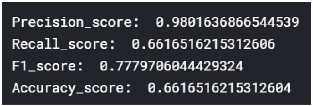
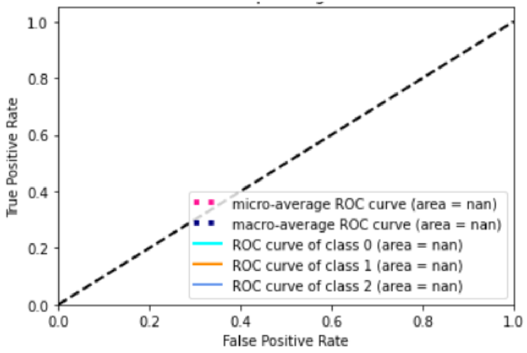
The reason for the coincidence of the ROC curve and the X-axis is that most of the predictions are zero. The reasons are as follows:

1. The two embedding methods, BOW and TF-IDF, do not work well as SVM, and even after normalizing the input word (frequency) vector matrix, most of the predictions are still the same.
2. The number of “neutral” labels in the sample is much higher than the number of “positive” and “negative” labels, which is also a problem in the sample selection process.
3. The parameters of SVM can be adjusted more precisely to make the classification better.

Instead of further tuning this model, we tried other algorithms first.

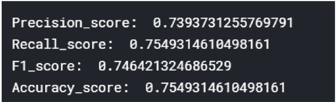
TF-IDF+SVM

The 38473-dimensional embedding of the TF-IDF derived posts is used as the input to the SVM in the sklearn package.

The source code is similar to the model above, so I will not repeat it here. The results are shown below.

The parameters are as follows.

clf = svm.SVC(C=0.8, kernel='rbf', gamma=20, decision_function_shape='ovr')

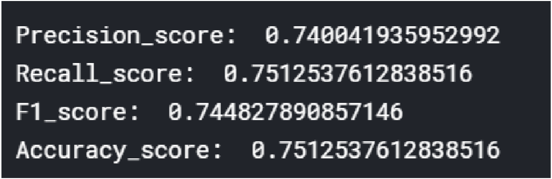
BOW + Decision Tree && TF-IDF + Decision Tree

The source code is similar to the model above, so I will not repeat it here.

Here’s the result for BOW + Decision Tree.

Here’s the result for TF-IDF + Decision Tree

Word2Vec + RNN

Embedding Weibo content using Word2Vec, then the resulting 400-dimensional vector is fed into a 102001 recurrent neural grid with one hidden layer.

Parameters:

batch_size = 100 
n_iters = 20000 
seq_dim = 20 
input_dim = 20 # input dimension
hidden_dim = 200 # hidden layer dimension 
layer_dim = 1 # number of hidden layers
output_dim = 3 # output dimension

So far we have obtained the embedding of all words, the key problem is how to represent the sentences. I referred to the information below and chose to try it with word2vec using Gensim.

At the first time we try, there is exploding gradient.

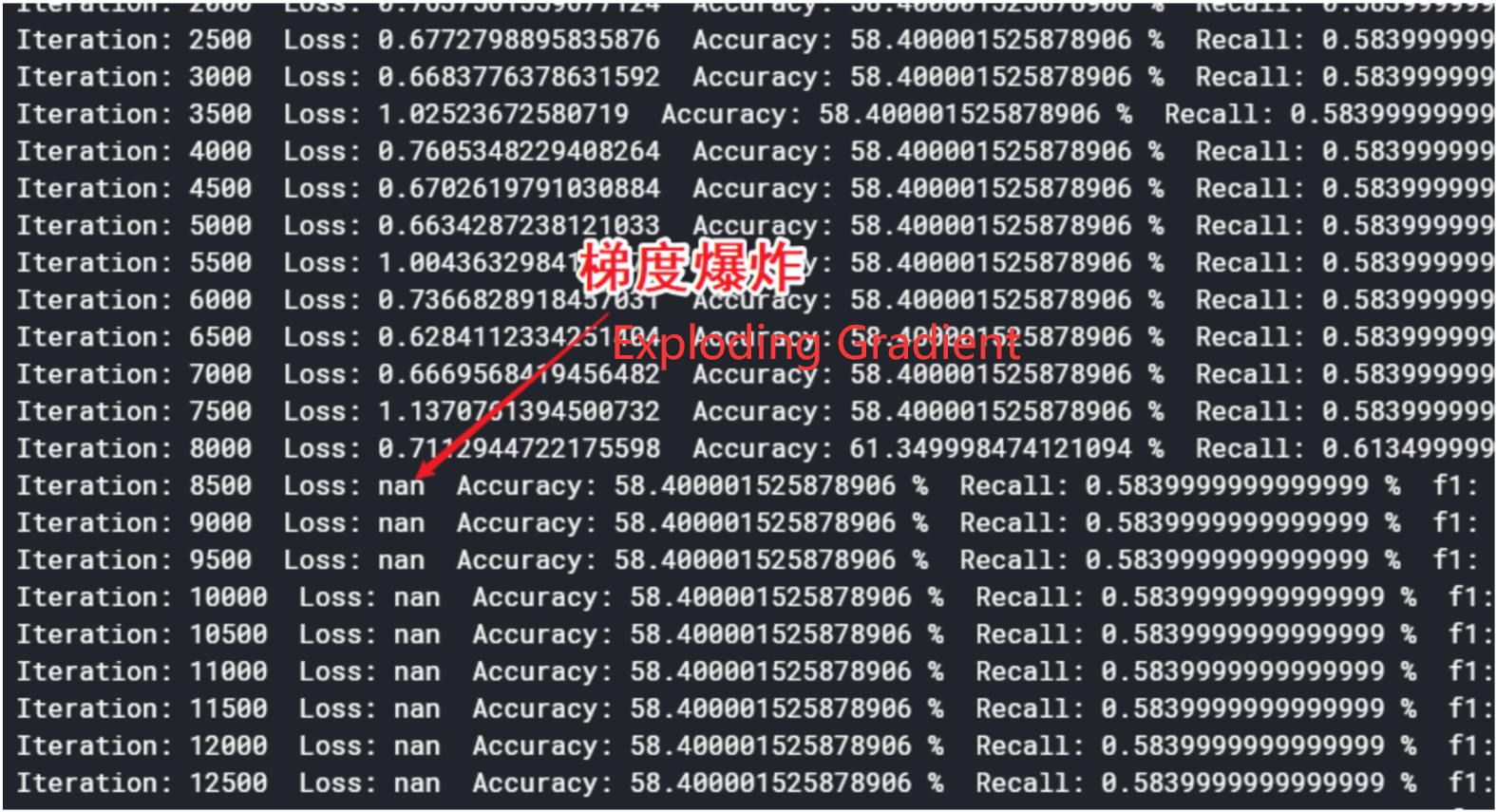
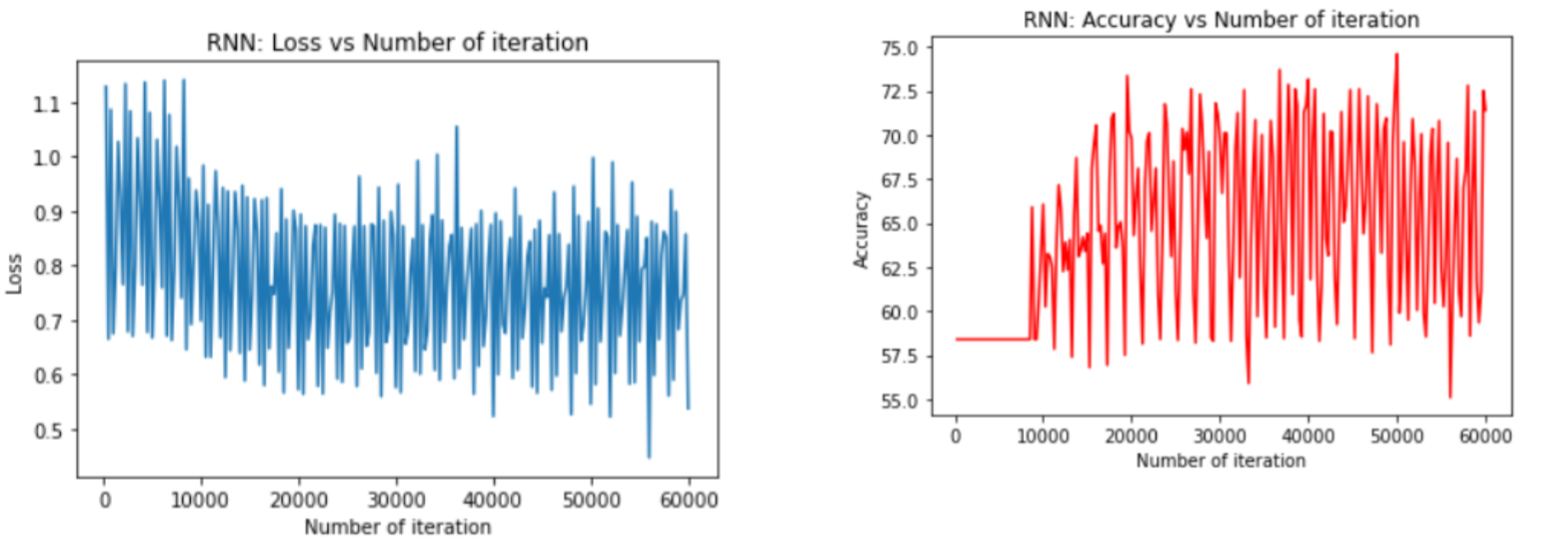
After adjusting the learning rate to 0.03, the results after 60,000 generations of training are shown below.

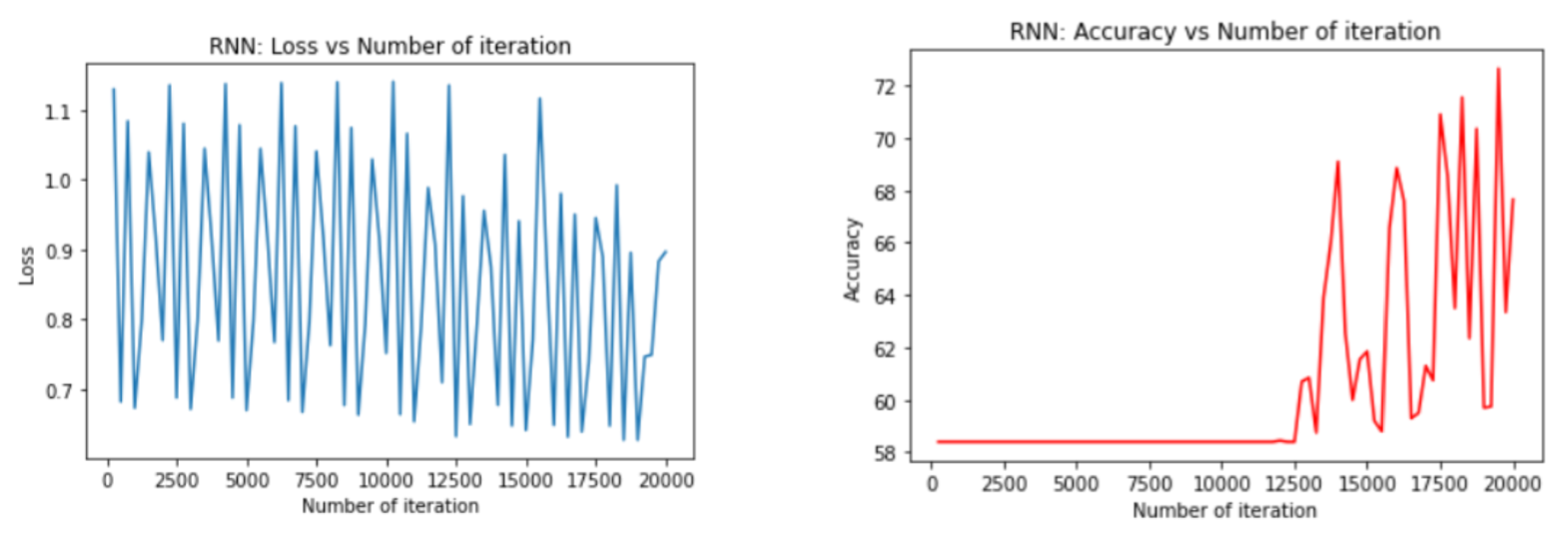
After adjusting hidden layers, the results after 20,000 generations are shown below.

Analysis of Results

This is a triple classification problem on the emotion of NLP. The results are shown as below.

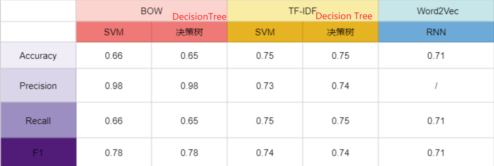
As can be seen from the above graphs, the SVM and Decision Tree algorithms have very little impact on the actual results, and the most important factor affecting the prediction results is the Embedding method. In this dataset, TF-IDF is more effective than BOW. In the end, the results of TF-IDF+SVM, TF-IDF+Decision Tree and Word2Vec+RNN are similar. The reasons for this result are as follows:

1. The original dataset is not evenly distributed, and there are more “neutral” comments than “positive” and “negative” posts, so in the predictive classification process, most of the postss are not evenly distributed. The majority of posts tend to be classified as “neutral” in the prediction classification process, which is of course consistent with the actual situation. This is why the Embedding method has a greater impact on the results than the classification method.
2. The dataset is not large enough. I thought that a data set of about 10,000 would take a lot of training time, but Kaggle can use GPUs and the CPU speed of Kaggle is not slow, so I could have done it directly with the original data set of 10W, and the result would be better.
3. Parameter optimization. It is only fair to use the optimal parameters of each model for comparison of results.