ICM 2021 | Social Network | Cracking the Secret of Musical Influence

We participated in ICM 2021 during Feb 5th - Feb 9th and finally honored Meritorious Winner(Top 7%)😆. Because we 3 people are all music enthusiasts, we chose the problem D about data mining in music similarity and influence. We thought we could do better in this field. It turns out that we were right. Here is our thinking and solution to this problem.

Topic and Datasets

Here are the topic and the datasets. You can also see them on COMAP.

In short, our team has been identified by an organization to develop a model that measures musical influence. This problem asks us to examine evolutionary and revolutionary trends of artists and genres. We has been given 4 data sets:

influence_data.csv represents musical influencers and followers, as reported by the artists themselves, as well as the opinions of industry experts. These data contains influencers and followers for 5,854 artists in the last 90 years.
full_music_data.csv provides 16 variable entries, including musical features such as danceability, tempo, loudness, and key, along with artist_name and artist_id for each of 98,340 songs. These data are used to create two summary data sets, including: mean values by artist - data_by_artist.csv, means across years data_by_year.csv.

Overview

Music has been a necessary part of human life and history since we human have consciousness. At the same time of human evolution, music is constantly changing new forms and contents. Music itself doesn’t evolve, and there’s no doubt that it’s done by a group of people called “artists”. It’s a common sense that a new form of music occurs under the action of many factors, such as artists’ innate creativity, current social or political events, access to new instruments or tools, or other personal experiences.

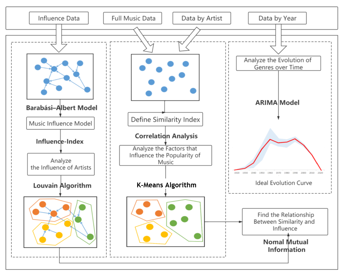
Figure 1: The architecture of our model

Based on some basic musical attributes, our aim in this report is to build a model to quantify musical evolution. We are expected to provide a measurement mechanism to observe how the previous music affects the later music and musicians. So two major models are established to finish that job.

For the model 1, we analyzed the relationships between genre, artist and music from the perspective of influence and similarity. We use the BA model to explain the influence network, which connects the influencers and followers. Based on the influence relationships between artists, we use the directed edge of the model to construct an influence-index. And then based on this index, we use the improved Louvain algorithm to in community partition to get The partition based on influence.

On the other hand, from the perspective of the similarity between artists, we use Pearson correlation coefficient to remove the redundant of music attributes, and construct the measure index of similarity. Based on this index, we use the improved K-Means algorithm in community partition, and finally obtain The partition based on similarity.

We creatively proposed to combine these two networks, and the NMI index is used to analyze the relationship between similarity and influence. Finally, we prove that the influencers actually affect the music created by the followers.

For the model 2, we took time into consideration. In order to analyze the musical evolution process, We use ARIMA model to create an ideal evolution curve. We compare the real curve with the ideal evolution curve to find how the social, culture and technology affect the music. We give an example of electronic music. Symbols and Definitions show in the Table 1.

Model 1: BA Model and Optimized Louvain-KMeans Algorithm

Model 1 we analyze social networks from the perspective of influence and similarity, and then analyze the influence and similarity relationship among genres, artists and music.

In this model, we use directed graph to construct influence network and BA model to explain the influence propagation relationship in the network. First, we analyzed the influence relationship between artists. We propose the influence index by using the indegree and outdegree parameters inthe directed graph, and use the improved Louvain algorithm in community partition to get the “The partition based on influence”.

Then we analyze the similarity among the music, we use Pearson correlation coefficient to delete redundant attributes, and propose the measure of “similarity”. Through similarity measurement, the improved KMeans algorithm is used in community partition to obtain “The partition based on “similarity”.

After that, we innovatively combine the above two networks, and perfectly explain the relationship between music influence and similarity by using NMI parameters. We call this innovative method Optimized Louvain KMeans Algorithm.

Analysis of Music Influence

The influence of network (BA model)

In Model 1 we analyze social networks from the perspective of influence and similarity, and then analyze the influence and similarity relationship between genres, artists and music.

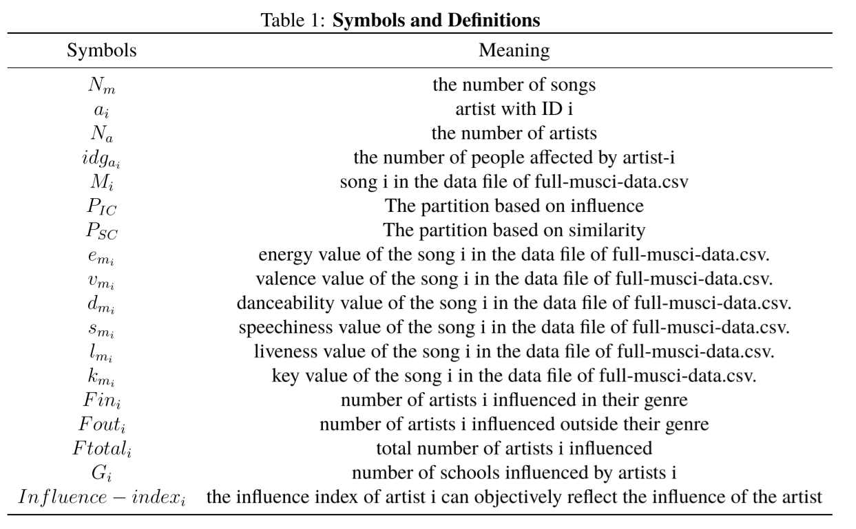
Influence_data.csv includes 5854 artists in the past 90 years according to the artists themselves and industry experts. We construct 42770 influence relationships among the 5854 artists through the data set, and the directed edges in the network point from the follower to the influencer. In the Figure3.1.1, artists of different genres are represented by different colors. There are 19 genres of music (except unknown) in the dataset.

Through the Figure2, we can roughly know the influence relationship between different genres. For example, we can easily see that Pop/Rock music has influence on all other genres, which is also determined by the characteristics of Pop/Rock music itself. Based on this network, the later content of this paper will further analyze the relationship between the influence of music characteristics and social network, age, policy and so on.

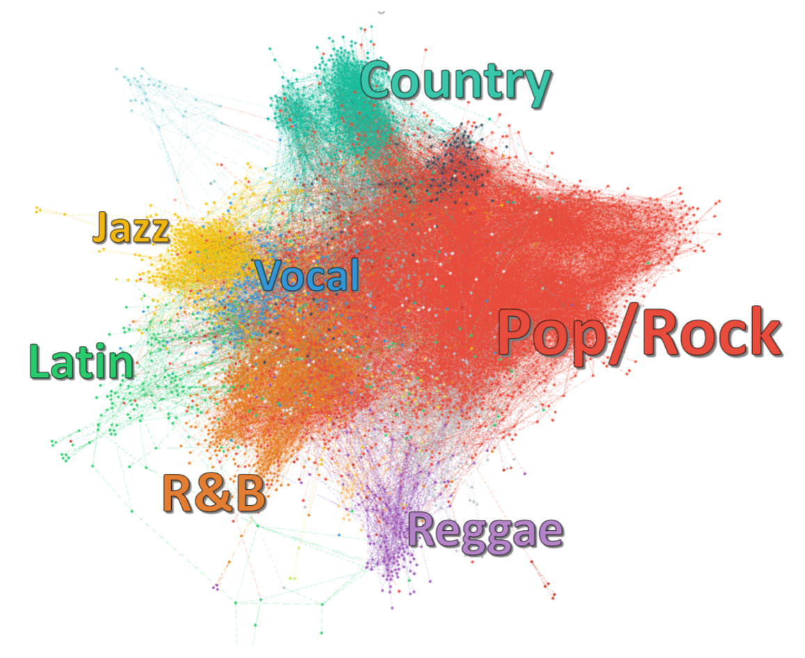
Figure 2: Directed network of musical influence

In network theory, scale-free network is a kind of complex network. Its typical feature is that most nodes in the network are only connected with a few nodes, and a few nodes are connected with a lot of nodes. In reality, many networks have scale-free characteristics, such as Internet, financial system network, social network and so on.

According to the influence direct graph, we guess that the influence network is a scale-free network, and then we will verify it by BA model.This model is based on two assumptions.

Growth model: many real networks are constantly expanding and growing, such as the birth of new web pages in the Internet, the publication of new papers and so on. Obviously, the musical influence network is also expanding through the increasing influence relationship.
Priority connection mode: when new nodes join, they tend to connect with nodes with more connections. For example, new web pages usually have connections to well-known Web sites, and new papers tend to cite well-known literatures that have been widely cited, etc. In reality, the same is true of influence. New musicians are more likely to be influenced by
influential influencers.

Based on the above two hypotheses, we randomly selected 500 followers from the data set, removed them from the established social network, and then connected them back to the influence network by building a scale-free network with BA model.

There are $Na$ nodes in the original network, we will add a new artist $a_i$ to the network. When $a_i$ is a new node, $m$ edges are connected from the new node to the original node, and the connection mode is the node with priority given to the high heights. For the original artist $a_j$ in the network,the number of degree in the original network is recorded as $idg{aj}$. Then the probability $p{a_i,a_j}$ of the new node can be canculate as follows:

$P_{a_i,a_j}=\frac{idg_{a_j}}{\sum_{K \in artist_{id}}idg_{a_k}} \tag{1}$

By choosing the appropriate probability threshold, we add these 500 nodes back to the influence network, and create related directed edges. According to the real influence network, we calculate the connection accuracy of each new node($a_i$) and the original node. The accuracy of the connection betweennew node($a_i$) and the original node is 81.74%. This shows that the influence network basically conforms to the BA model.

According to the properties of BA model, we can know that the distribution of the number of the followers of artists can be approximately described by a power function with a power exponent of 3. For artist $a_i$, the distribution function of the number of people affected is:

$p(idg_{a_i}) \propto 2idg^3_{a_i} \tag{2}$

The distribution function can help us better explain the spread of influence, and can also be used to predict which artists are more attractive to the new artists.

Analysis of music influence from the perspective of genre

To quantify the influence of music genres, based on the previous social network, we counted the number of directed edges between genres as the influence parameter, and built the heat map between genres. In order to show the heat map better, we take logarithm of the number of directed edges.

As can be seen from the below Figure 3, the influence of all artists is mainly reflected in the genre itself. Jazz has an impact on all other genres of music. Pop / Rock, R&B and Vocal also have a great impact on other fields.

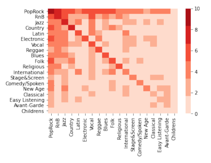
Figure 3: Heat map between genres

Influence-index

In order to evaluate the music influence of artists better, we introduce the following evaluation measures. On the basis of the number of followers, we construct the comprehensive measure of influence index, which combines the influence of artists in and out of their genres to give an objective evaluation of the influence of artists.

$Influence-index_i=F_{in_i}+logG_i * F_{out_i} \tag{3}$

We choose pop / rock artists as a sub network to investigate the influence of all artists. According to the influence index we set, we find out the top ten artists of this genre.The music genres and influence-index influenced by the ten artists are shown in the following table.

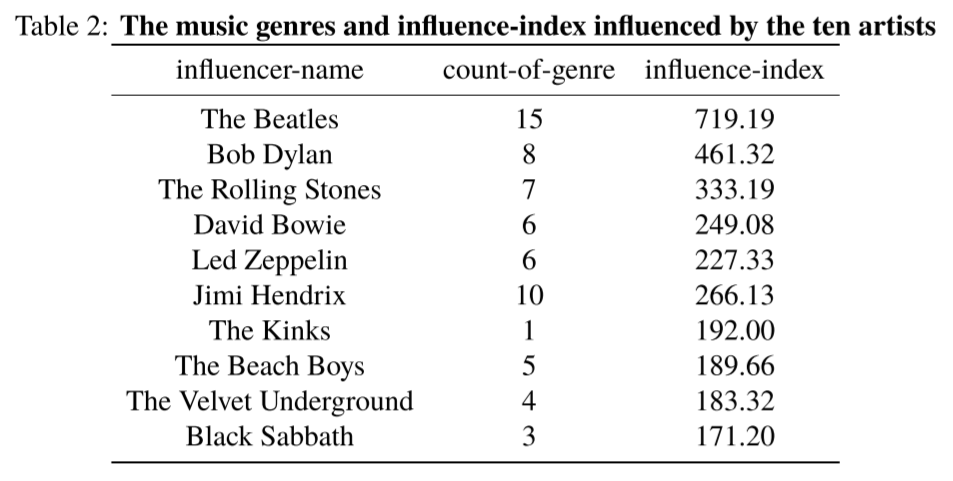
It is easy to check the influencer and followers of each artist in the network we built. Taking The Beatles as an example, the influence network chart of its music is shown in the Figure 4.

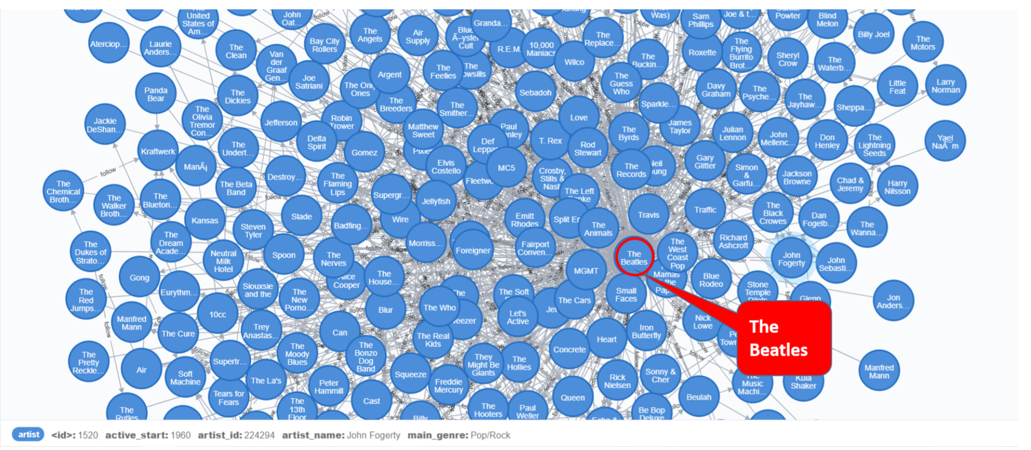
Figure 4: The influence network chart of The Beatles

Analysis of Music Similarity

The similarity index

In order to establish the music similarity measurement model, we can compare the similarity degree of each parameter between different music. In this question, there are 7 characteristics of the music and 5 types of vocals, a total of 12 parameters to reflect the characteristics of music (danceability, energy, valence, tempo, loudness, mode, key, acousticenss, instrumentalness, livenss, speechiness, explicit).

By calculating Pearson correlation coefficients between 12 music parameters, the correlation co-efficient matrix is obtained, and the redundant parameters with high correlation can be eliminated.

Energy and valence data in full-music-data.csv were taken as an example to calculate the correlation coefficient, and the data could be expressed as: $ e:\{e{m_1}, e{m2}, e{m3}, …, e{m{N_n}}\} $, $ v:\{v{m1}, v{m2}, v{m3},…, v{m_{N_n}}\} $.

$\begin{align} &Mean Value: E(e) = \frac{\sum_{i=1}^ne_{m_i}}{n}, E(v)=\frac{\sum_{i=1}^nv_{m_i}}{n}, \\ &Covariance: Cov(e, v) = \frac{\sum_{i=1}^n(e_{m_i}-E(e))(v_{m_i}-E(v))}{n}, \\ &Standard Deviation: \delta_e=\sqrt{\frac{\sum_{i=1}^n(e_{m_i}-E(e))^2}{n}}, \delta_v=\sqrt{\frac{\sum_{i=1}^n(v_{m_i}-E(v))^2}{n}}, \\ &Pearson = \rho_{ev} = \frac{Cov(e, v)}{\delta_e\delta_v}=\frac{\frac{\sum_{i=1}^n(e_{m_i}-E(e))(V_{m_i}-E(v))}{\delta_e\delta_v}}{n} \end{align} \tag{4}$

Using the data in full-music-data.csv, the correlation coefficient between each index can be calculated. Its correlation coefficient matrix is shown in Figure 5.

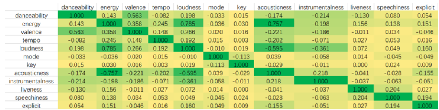
Figure 5: The correlation coefficient between each index

In order to reduce the influence of the correlation between indicators, indicators in each group with the absolute value of correlation coefficient greater than 0.3 were selected. Then, one of the two indicators of each group was selected, and the index used to evaluate music similarity was as follows:danceability, energy, mode, key, liveness, speechiness and explicit.

The values of mode and explict are Boolean values, so they are excluded from the music similarity model. The similarity of songs was evaluated by comparing the degree of differentiation of the remaining five indicators between different songs. We defined a numerical quantity called similarity to indicate the degree of difference between songs, and the higher the similarity value is, the more similar the songs are.

For example, calculate the similarity of song j and song k in full-musci-data file, and its data can be expressed as: $Mj{d{mj}, e{mj}, l{mj}, s{mj}, k{mj}}, M_k{d{mk}, e{mk}, l{mk}, s{mk}, k{m_k}}$.
The similarity of the two songs is defined as:

$def: Similarity = \frac{1}{\sqrt{(d_{m_j}-d_{m_k})^2+(e_{m_j}-e_{m_K})^2+...+(k_{m_j}-k_{m_k})^2}} \tag{5}$

Similarity analysis between music genres

We selected 12 music genres in the data set to analyze their music similarity. For each genre, we selected 50 artists with the highest influence index, and calculated the music style similarity between these 500 artists. Then the music similarity between different genres is calculated according to the same genre and different genres. The results are shown in the Figure 6 below.

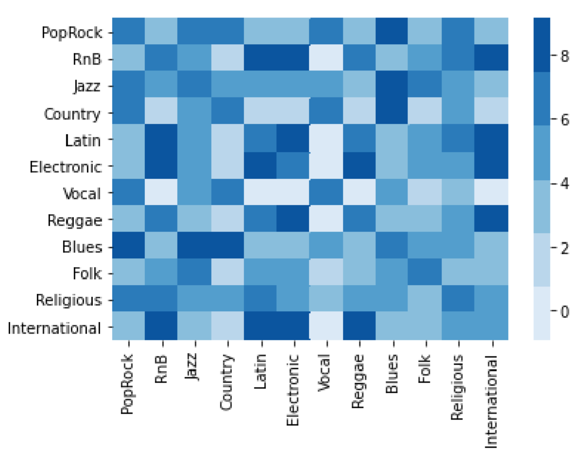
Figure 6: Music similarity between different genres

The darker the color in the figure 6 is, the higher the similarity between genres. For example, the similarity between Blues and Pop/Rock,jazz and Country is very high, while the similarity between R&B and Vocal is very low. Similar conclusions can be drawn directly from the figure.

In order to better distinguish the characteristics of music genres, we use radar chart to intuitively show the prominent characteristics of each genre.The musical characteristics of these 12 genres are shown in the Figure 7.

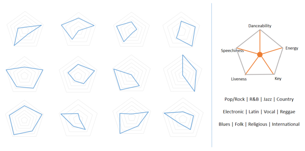
Figure 7: Music characteristics

The analysis of the factors that influence the spread of music

Using the data, the correlation coefficients between 12 indexes and the popularity of music are calculated.

In this question, we assume that if the absolute value of the correlation coefficient is greater than 0.3, we can think that there is a strong correlation between the data. When the absolute value of the correlation coefficient is between 0.1 and 0.3, we can think that there is a correlation between the data.

The characteristics of music communication can be reflected from the popularity of music, so from the correlation coefficient, it can be concluded that the communicability of music is positively correlated with the dancebility, energy, loudness and explicit, and negatively correlated with the instrumental, acoustic and other indicators, and is most affected by the dancebility, loudness and acoustic.

Optimized Louvain-KMeans Algorithm and NMI

Through the heat map of influence and similarity, we can qualitatively observe the relationship between music influence and similarity.

Next, we innovatively propose the optimized louvain-kmeans algorithm to quantitatively analyze the relationship between music influence and similarity with the help of NMI.The architecture of this model is shown in the figure 8.

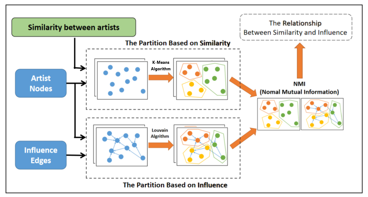
Figure 8: Flow chart of the model

The community partition based on influence

The Louvain method for community detection is a method to extract communities from large networks created by Blondel et al. from the University of Louvain (the source of this method’s name). The method is a greedy optimization method that appears to run in time $O(n · log_2n)$ if $n$ is the number of nodes in the network.We will use the Louvain algorithm to divide the influence network.

Before using Louvain, we need to introduce the concept of modularity. We use the Louvain algorithm to make as many edges as possible in the community and as few as possible between the communities. The measure of this index is modularity.

The number of nodes in the network is $Na$, the number of edges is $N{infl}$, and the indegree of node $ai$ is $idg{ai}$. The adjacency matrix of the network is expressed as A, $A{a_i,a_j}=0$ means there is no edge between $a_i$ and $a_j$. $AVW = 1$ means there are edges between the two nodes.

Define variable s, and $s{a_ia_j}$ means that $a_i$ and $a_j$ belong to the same partition. $s{aia_j}=-1$ means that the two nodes belong to different partition. Then we can use $\delta{aia_j} = 1/2(s{a_ia_j} + 1) $ to verify if $a_i$ and $a_j$ belong to the same partition in a quantitive way. If the result equals one, we can say the two nodes belong to the same partition. If not, the result equals zaro. Then the probability expectation of modularity can be expressed as:

$\overline{Q} = 1/2\frac{\sum_{a_ia_j}A_{a_ia_j}}{N_{infl}} \delta_{a_ia_j} \tag{6}$

Modularity can be finally expressed as:

$Q=\frac{1}{2m}\sum_{a_ia_j}(A_{a_ia_j}-\frac{idg_{a_i}idg_{a_j}}{2N_{infl}})\delta_{a_ia_j} \tag{7}$

Through greedy algorithm, the modularity is continuously optimized to achieve “community partition based on influence”,The schematic diagram of the improved Louvain algorithm is shown in the Figure 9.

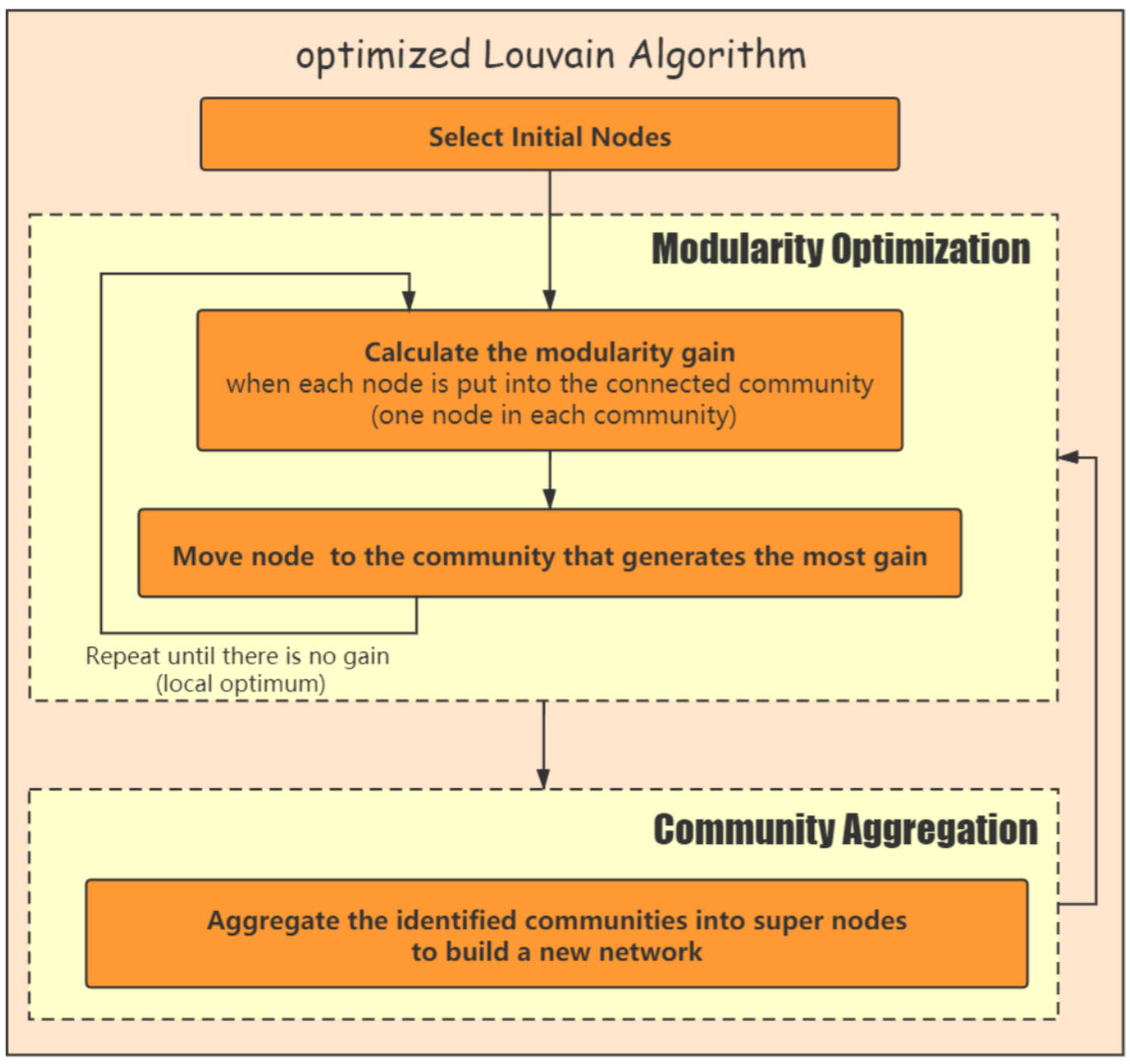
Figure 9: Optimized louvain algorithm

In the process of optimization, we select the artist with the biggest influence factor among 19 music genres, and prevent them from being divided into a module, so as to improve the efficiency of community partition. The community partition results are shown in the Figure 10.(different colors represent different communities)

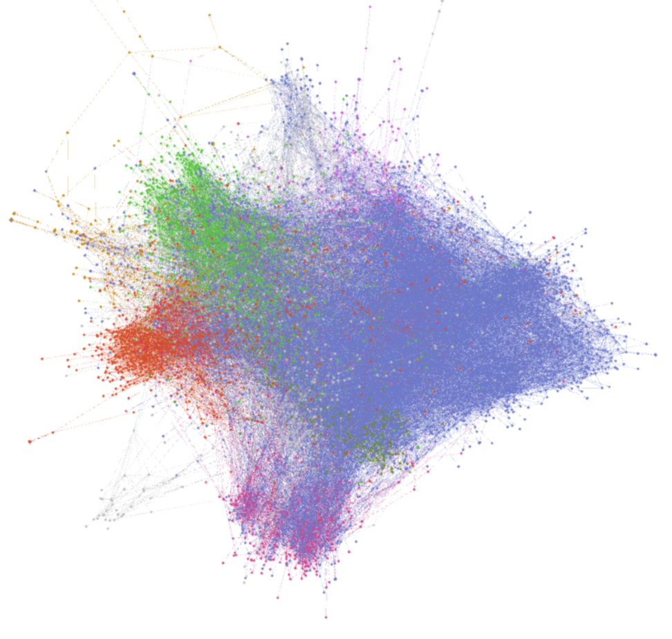
Figure 10: The partition based on influence

The communiy partition based on similarity

We use KMeans to divide all the artist nodes into communities, so that the music similarity within the community is higher, and the music similarity between the communities is lower. Similar to the Louvain algorithm, we use the artist with the largest influence factor in the same 19 music genres, and prevent them from being divided into a module, so as to improve the efficiency of community partition.The community partition results are shown in the Figure 11(different colors represent different communities)

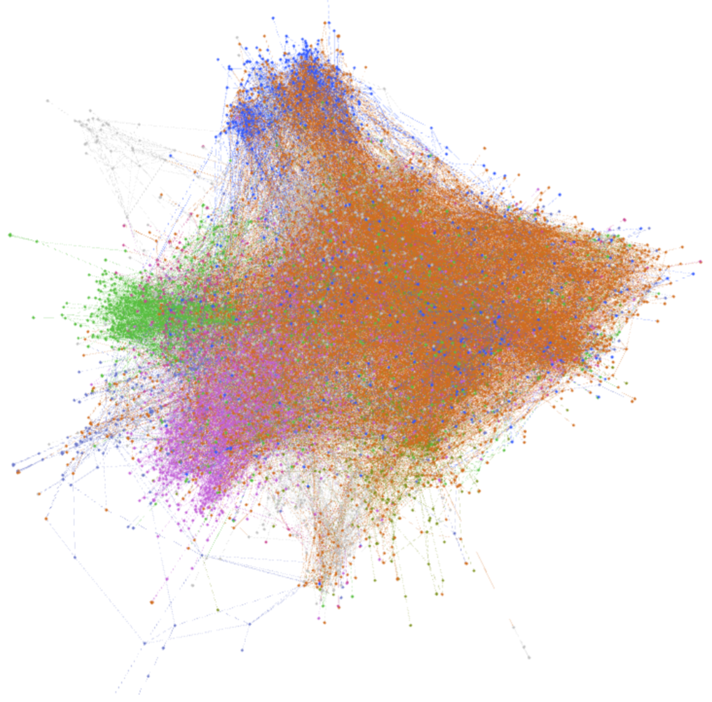
Figure 11: The partition based on similarity

The relationship between influence and similarity was analyzed through NMI

NMI is often used to detect the difference between the results of the partition and the true partition of the network and calculate the correct rate. Here we use the NMI index to evaluate the similarity between the influence-based and similarity-based social partitions.The higher the NMI index is, the more similar the two partitions are, which indicates that the influencers actually affect the music created by the followers.

In our model,$P{SC}$ stands for “similarity-based community partition” and $P{IC}$ for “influence-based community partition”, and the NMI index of these two can be expressed by the following formula:

$\mathrm{NMI}=\frac{-2 \sum_{i=1}^{C_{P_{I C}}} \sum_{j=1}^{C_{P_{S C}}} C_{i j} \cdot \log \left(\frac{C_{i j} \cdot N}{C_{i} \cdot C_{j}}\right)}{\sum_{i=1}^{C_{P_{I C}}} C_{i} \cdot \log \left(\frac{C_{i}}{N}\right)+\sum_{j=1}^{C_{P S C}} C_{i j} \cdot \log \left(\frac{C_{j}}{N}\right)} \tag{8}$

where N is the number of nodes, C is a confusion matrix, the element $C{ij}$ in the matrix indicates the number that the nodes belonging to the community i in the SC partition also belong to communities j in the IC partition. $P{IC}(P_{SC})$ is the number of communities in IC(SC) partition, $C_i(C_j)$ is the sum of elements in matrix C. The grater the value of NMI,the more similarity between SC and IC partition, when the NMI value is 1, it indicates that SC and IC are the same partition of the network.

Finally, the NMI value we calculated is 0.6237, indicating that the influencers actually affect the music created by the followers.

Model 2: Time-Series Analysis

It is a normal process that music genres emerge, evolve, and disappear. Our team member managed to observe big turns over time, and identify the key revolutionary artist of each genre. Whenever a music genre is about to leap, there will always be clues to change. As for a music genre, it is obvious that the explosive growth in the number of new artists and new songs indicates the prevalence and significant leap of the genre. So our team counted the number of artists and songs in the history of ten major music genres, and found the time of change in the visual image. According to the influence network, the most influential artists in these years were identified as the pioneers of the music revolution, that is, the so-called music revolutionaries. The details are shown below.

The evolution of genres over time

We have studied the evolution of ten genres over time. In the text, we choose Jazz, R&B and Country as three genres to illustrate their evolution over time.

New Artists

First of all, look at the number of artists added from the genre.According to the data given, the statistical changes of the number of people in the three schools from 1930 to 2010 are shown in Figure 12.

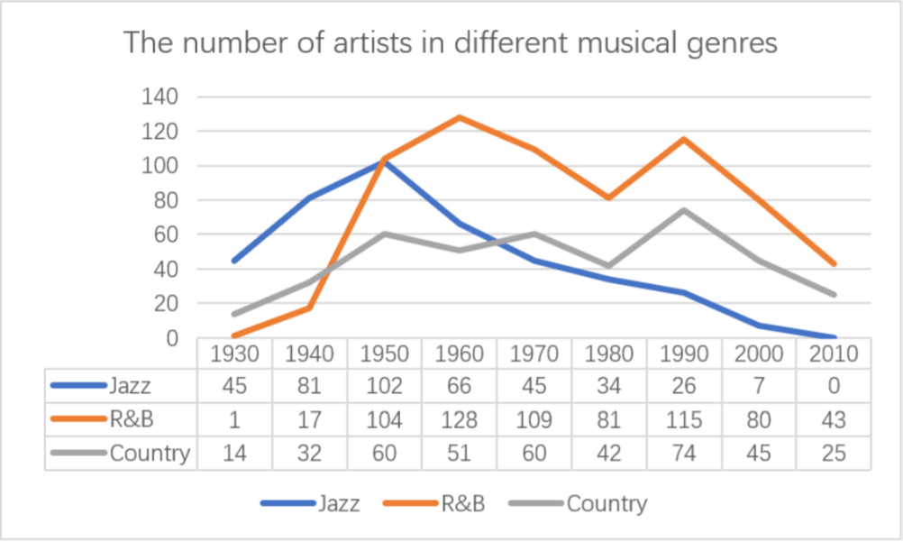
Figure 12: The number of artists in different musical genres

It can be seen from the figure that jazz, R&B and country all rose in the United States in the 1930s. Jazz flourished from the 1930s to the 1950s, and the number of new artists reached 102 in the 1950s. After the 1950s, jazz began to decline rapidly, and the number continued to decline. By the 2010s, there was no jazz New artists are included in the statistics.

R&B music developed slowly from 1930’s to 1940’s, and the number of artists increased slowly. However, as time went into 1940’s, R&B music genres developed rapidly, and the number of new artists increased from 17 in 1940 to 104 in 1950 in just 10 years. When R&B developed into 1950s, the number of artists still maintained a steady growth momentum, and reached the peak in 1960 From the 1960s to the 21st century, R&B declined as a whole. The number of new artists has been decreasing except for the growth in the 1980s. In 2010, the number of new artists fell back to the level of the early 1940s.

The number of artists in the country music genre increased slowly, showing a fluctuating upward trend from 1930 to 1990. The number of new artists reached the peak of 74 in 1990. However, compared with the peak of jazz and R& B genre, the number of artists was still small. After 90 years, the country music genre began to decline, and the number of new artists fell back to the
beginning of the genre The number of musicians.

The release of songs

In terms of the number of songs released, in the data used, we exclude the songs jointly released by multiple artists, and all the songs included in the calculation are published by artists alone, which can avoid that a song may be released by artists of multiple genres.

According to the given data, the changes of the number of songs released by the three genres from 1920 to 2020 are counted, as shown in Figure 13.

Compared with the broken line trend in Figure 1 and Figure 2, we can conclude that the increase of new generation artists will significantly affect the number of songs released, and this effect is often ahead of the increase in the number of songs released, and there is a cumulative effect. Taking jazz music genre as an example, the number of new generation artists in the genre was at a high growth level from 1930 to 1960. In 1950, the number of new generation artists reached its peak. During this period, the genre accumulated a large number of excellent artists. These artists matured in the 1950s and 1960s, and a large number of music works emerged. During this period, the music circulation of jazz music was much higher than that of any other period, reaching the peak of 486 songs in 1957. The same is true of R&B music. In 1960, the number of new generation artists
reached its peak, and then in 1972, the number of R&B music released reached its peak of 339.

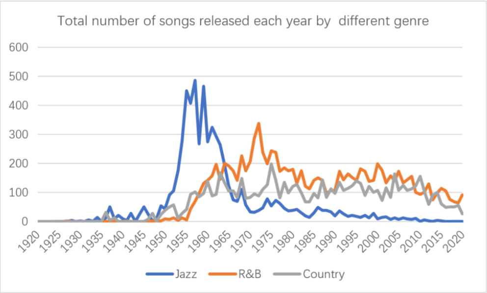
Figure 13: Total number of songs released each year by different genre

Genre popularity

From the perspective of popularity, we first give the definition of genre popularity. Gene popularity: based on the active-Start, the arithmetic mean value of the popularity of all artists of the same genre is defined as genre popularity.

For example: jazz music genre, active- There are 45 artists who started in 1930, according to the data table-by-artist.csv We can know the popularity value of artists who meet the conditions, and we can get the popularity of jazz music in 1930 by taking the arithmetic average of these values.

According to the above definition, we can get the change curve of the three genres from 1930 to
2010, as shown in Figure 14.

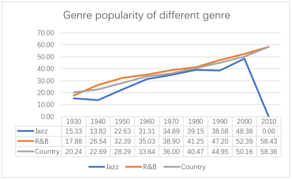
Figure 14: Grnre popularity

From the trend of the line chart, the value of Genre popularity is increasing over time. The reason for the decline of jazz curve from 2000 to 2010 is the lack of 2010 active-Start’s Jazz artist data, so its value was zero in 2010. Because the popularity of songs is calculated by algorithm, and the result largely depends on the total number of tracks played and the time of the most recent track played. Generally speaking, as time goes on, the frequency of playing the track will increase significantly, and it has a higher popularity. Therefore, the popularity of genres will increase with
the passage of time.

The influence of external factors on the development trend of genres

We divide the ideal evolution of music genres into four stages: initial stage, development stage, booming stage and recession stage. We use the number of songs of a genre in a certain period to express the prosperity of the genre in that period. Based on the number curve of 10 genres, we use ARIMA model to fit an ideal evolution curve of genres.

Without the influence of social environment, scientific and technological development and other factors, genres will evolve according to the ideal curve.

ARIMA model(Auto regressive Integrated Moving Average model ) is one of the time series prediction methods. In ARIMA (P, D, q), AR is “autoregressive”, P is the number of autoregressive terms; Ma is “moving average”, q is the number of moving average terms, and D is the difference order of making it a stationary sequence.

The ideal evolution curve of genres fitted by this model is shown in the Figure 15 (the light blue area is the error range). Compared with the ideal evolution curve and the actual evolution curve of music genre, when there is a significant difference between the two in a certain period, it shows that there are social and cultural factors that have a great impact on the genre at this time.

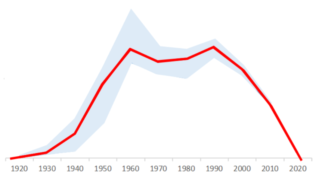
Figure 15: The ideal evolution curve of genres

Taking electronic music as an example, the evolution curve of electronic music and the evolution curve of the genre in the ideal state are shown in the Figure 16.

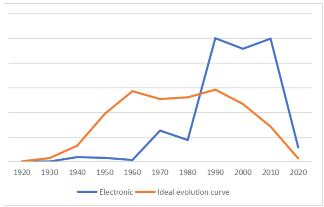
Figure 16: The evolution curve of electronic

In fact,following the emergence of raving, pirate radios, and an upsurge of interest in club culture. Electronic music achieved widespread mainstream popularity in Europe. Meanwhile, MIDI devices, which has been the musical instrument industry standard interface since the 1980s through to the present day, became commercially available in 1980s.These cultural and technological factors have promoted the rapid development of electronic music.

Conclusions

To understand and measure the influence of previously poducted music on new music and musical artists, we proposed a series of novel models to address the sub-issues from creating the influence network based on the similarity between artists. The proposed model achieves high accuracy and robustness.

We create the directed network based on music influence and use BAmodel to explain how the influence network expend. Thenwe propose Influence-Index to analyze the influence between genres and artists. We select the most 10 influential artists and show their influence-index.
In order to analyze the similarity between genres, artists and music, we use correlation analysis to remove redundant attributes. We finally select 7 attributes which actually infect the similarity. They are danceability, energy, key, liveness, speechiness, mode and explicit. Based on these attributes, we propes similirity index.
To find the relationship between the music similarity and the influence, we propose a Optimized LOUVAIN-KMeans Algorithm and use it to community partition. By participating artists into different community through Louvain algorithm and KMeans algorithm, we can obtain 2 different partition. Then we use NMI to estimate the similarity between these 2 partions. Finally we get the conclusion that influencers actually affect the music created by followers.
We analyze the influence processes of musical evolution that occoured over time. We use ARIMA model to create an ideal evolution curve. By comparing with the ideal evolution curve, we can find how the social, culture and technology affect the music. We give an example about electronic music.

Strength and weaknesses

Strengths

-We creatively proposed Optimized LOUVAIN-KMeans Algorithm and use the partition to explain the relationship between the influence and music similarity. The community network is as a bridge between them, and the model can reflect the relationship effectively.

We proposse Influence-Index to estimate the influence of the artists objectively. It’s not accuracy to use only the number of followers or the number of music.
When analyzing the similarity between music and artists, our model is simple and convenient. Among the 12 music attributes given in the original data set, we remove the redundant attributes through correlation analysis, so that our model can calculate the similarity more efficiently and maintain a higher accuracy.
We creatively use ARIMA model to generate an ideal evolution curce of the genre. It make our model more robust, and can be used in many other situation. The ideal evolution curve reveal the process of the evolution in these genres.

Weakness

We don’t consider the influence between genres when we construct the ideal evolution curve. And new genres will appear at any time, so the curve may not that accuracy.
The interpretability of the influence and similarity model is not strong. We only find the relationship between similarity and influence. But we don’t know how it operates indetail.
The amount of data of some minority genres is too small, the prediction result of the model for minority genres is not good.

This work is licensed under a Creative Commons Attribution-NonCommercial-ShareAlike 4.0 International License