Predicting the price by its description | ML Algorithms

This is a task in the course Introduction to Data Science. Our team was going to predict the price of products by their description.

Topic

Background

Considering the number of products sold online, product pricing becomes more difficult at scale. Apparel has strong seasonal pricing trends and is heavily influenced by brands, while electronics prices fluctuate based on product specifications. It is a meaningful question to help merchants effectively sell their goods by making reasonable pricing based on past information.

Target

The product description, product category and brand information is given and combined with the product price from the training data to set the price for the new product.

Obviously Versace’s clothes should be much higher in price than Metersbonwe’s clothes, and in the description of the goods, you can find a slight difference between the two descriptions.

This project aims to analyze the text information, extract the important information from the text information and derive the potential relationship with the price。

Analysis of atributes

Dataset

train.csv training dataset (Include price)
test.csv test dataset (Not include price) ; label_test.csv (Corresponding to the price of the test dataset)
f_test.csv Final measurement data set (Not include price)

Evaluation Indicators

We used Mean Squared Logarithmic Error (MSLE) to evaluate the algorithm:

$MSLE = \cfrac{1}{n}\sum_{i=1}^n(log(p_i+1)-log(\alpha_i+1))^2 \tag{1}$

Which $n$ means the number of samples in test dataset; $p_i$means the predicting price of sales; $\alpha_i$ means the real price.

Data Process

Learning sample code

The sample code given was first tried to understand the general idea of solving this problem. The main processes to solve this price prediction problem are: importing data and data exploration, data pre-processing, model construction, price prediction and measurement.

import data and exploration

Import the data and get acknowledge with it.

train_data = pd.read_csv('../data/4/train.csv', sep="\t")
test_data = pd.read_csv('../data/4/test.csv',sep='\t')
train_data.info()

<class 'pandas.core.frame.DataFrame'>
RangeIndex: 300000 entries, 0 to 299999
Data columns (total 8 columns):
train_id             300000 non-null int64
name                 300000 non-null object
item_condition_id    300000 non-null int64
category_name        298719 non-null object
brand_name           171929 non-null object
price                300000 non-null float64
shipping             300000 non-null int64
item_description     300000 non-null object
dtypes: float64(1), int64(3), object(4)
memory usage: 18.3+ MB

Data Preprocess

First of all, we need to remove price from the training data, and then remove train_id or test_id which are not useful. By looking at the data attributes above, we can see that category_name and brand_name have missing data, so the sample code is filled with missing directly.

def featureProcessing(df):
    # delete the data that will not be used
    df = df.drop(['price', 'test_id', 'train_id'], axis=1)
    # deal with the missing value with a default value
    df['category_name'] = df['category_name'].fillna('missing').astype(str)
    df['brand_name'] = df['brand_name'].fillna('missing').astype(str)
    df['item_description'] = df['item_description'].fillna('No')
    # convert the data : int -> str
    df['shipping'] = df['shipping'].astype(str)
    df['item_condition_id'] = df['item_condition_id'].astype(str)

    return df

Model Construction

First of all, the input of the model is done and the matrix of word frequencies is generated by CountVectorizer and TfidfVectorizer. Tfidf is better because the number of occurrences of each word in all field clocks is taken into account and the generated word frequency matrix is weighted.

vectorizer = FeatureUnion([
    ('name', CountVectorizer(ngram_range=(1, 2), max_features=50000, preprocessor=build_preprocessor_1('name'))),
    ('category_name', CountVectorizer(token_pattern='.+', preprocessor=build_preprocessor_1('category_name'))),
    ('brand_name', CountVectorizer(token_pattern='.+', preprocessor=build_preprocessor_1('brand_name'))),
    ('shipping', CountVectorizer(token_pattern='\d+', preprocessor=build_preprocessor_1('shipping'))),
    ('item_condition_id', CountVectorizer(token_pattern='\d+', preprocessor=build_preprocessor_1('item_condition_id'))),
    ('item_description', TfidfVectorizer(ngram_range=(1, 3),max_features=100000, preprocessor=build_preprocessor_1('item_description'))),
])

Predict the price by Ridge Regression.

def ridgeClassify(train_data, train_label):
    ridgeClf = Ridge(
        solver='auto',
        fit_intercept=True,
        alpha=0.5,
        max_iter=500,
        normalize=False,
        tol=0.05)
    # Training
    ridgeClf.fit(train_data, train_label)
    return ridgeClf

By understanding the dataset and studying the sample code, we learned that there are three angles to start with to optimize the answer to this question.

data preprocessing: How to handle missing values? How should the attributes be combined?
optimization when forming the word frequency matrix: adjusting the parameters of CountVectorizer and TfidfVectorizer.
Model selection and optimization: try models other than ridge regression, adjust model parameters.

Try more models

In the sample code above, the result obtained using the ridge regression model is about 3.01. After the hints from the previous class and the online search, we are ready to try the MLP model and the Lgmb model again. After roughly trying both models, we decided to further optimize the model using MLP.

`MLP`

The result of MLP is 0.4430 (MSLE)

`LGBM`

The result of Lgbm is 0.2688 (MSLE)

`MLP` Combined with `LGBM`

<1> Preprocessing

Import the data

train = pd.read_csv('data/train.csv', sep='\t')
test = pd.read_csv('data/test.csv', sep='\t')
# train and test data are handled together
df = pd.concat([train, test], axis=0)

Handling missing value

# Handling missing values
   df['category_name'] = df['category_name'].fillna('MISS').astype(str)
   df['brand_name'] = df['brand_name'].fillna('missing').astype(str)
   df['item_description'] = df['item_description'].fillna('No')
   # modifying data structure
   df['shipping'] = df['shipping'].astype(str)
   df['item_condition_id'] = df['item_condition_id'].astype(str)

Feature vectorization

Use the CountVectorizer class in the sklearn library to vectorize the text features and use FeatureUnion for feature union.

vectorizer = FeatureUnion([
        ('name', CountVectorizer(
            ngram_range=(1, 2),
            max_features=100000,
            preprocessor=build_preprocessor('name'))),
        ('category_name', CountVectorizer(
            token_pattern='.+',
            preprocessor=build_preprocessor('category_name'))),
        ('brand_name', CountVectorizer(
            token_pattern='.+',
            preprocessor=build_preprocessor('brand_name'))),
        ('shipping', CountVectorizer(
            token_pattern='\d+',
            preprocessor=build_preprocessor('shipping'))),
        ('item_condition_id', CountVectorizer(
            token_pattern='\d+',
            preprocessor=build_preprocessor('item_condition_id'))),
        ('item_description', TfidfVectorizer(
            ngram_range=(1, 3),
            max_features=200000,
            preprocessor=build_preprocessor('item_description'),
            stop_words='english')),
    ])

<2> Model Construction

The features were trained using the ridge regression model, the Lgbm model and the mlp model, respectively, and the solutions obtained in local tests were 3.01, 3.00, and 0.26, respectively.

Ridge Regression


def ridge_classify(train_data,train_label):
    #model
    model = Ridge(
            solver='auto',
            fit_intercept=True,
            alpha=0.4,
            max_iter=100,
            normalize=False,
            tol=0.05)
    #training
    model.fit(train_data, train_label)
    return model

lgbm Model

def lgbm_classify(train_data,train_label):
    params = {
        'learning_rate': 0.75,
        'application': 'regression',
        'max_depth': 3,
        'num_leaves': 100,
        'verbosity': -1,
        'metric': 'RMSE',
    }

    train_X, valid_X, train_y, valid_y = train_test_split(train_data, train_label, test_size=0.1, random_state=144)
    d_train = lgb.Dataset(train_X, label=train_y)
    d_valid = lgb.Dataset(valid_X, label=valid_y)
    watchlist = [d_train, d_valid]

    model = lgb.train(params, train_set=d_train, num_boost_round=2200, valid_sets=watchlist, \
                      early_stopping_rounds=50, verbose_eval=100)
    return model

mlp Model

The MLP model consists of two fully connected layers and a dropout layer, which is essentially a network of multiple hidden layers.

def mlp_model(train_data,train_label,row_train):
    model = Sequential()
    # fully connected layer
    model.add(Dense(64, input_shape=(row_train,), activation='relu'))
    # DropOut layer
    model.add(Dropout(0.4))
    # fully connected layer + classifier
    model.add(Dense(1, activation='relu'))

    model.compile(loss='mean_squared_logarithmic_error',
                  optimizer='adam',
                  metrics=['accuracy']
                  )

    model.fit(train_data, train_label,
              batch_size=300,
              epochs=1,
              )

    return model.predict(X_test)

Optimization when forming word frequency matrix

In the sample code we tried to replace all CountVectorizer with TdidfVectorizer and then use the Ridge model for prediction, but the result is not much optimized, only up to 2.9.
Later, when using the MLP, we completely discarded the CountVectorizer and used only the TdidfVectorizer.

Optimize the data pre-processing process

The way we optimize the MLP, which is basically perfected above, is to try different combinations of features.

Analysis of the attributes

First I analyzed the attributes:

item_condition_id    300000 non-null int64
shipping             300000 non-null int64

name                 300000 non-null object
category_name        298719 non-null object
brand_name           171929 non-null object
item_description     300000 non-null object

item_condition_id and shipping are considered directly as inputs, while name, category_name, brand_name, item_description are considered for different combinations to try.

Before that, we found an example tutorial on data visualization to analyze the attributes of the data.
The optimal combination of inputs is obtained by observing the data.

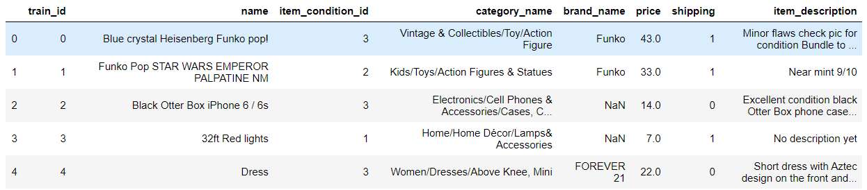
train.head()

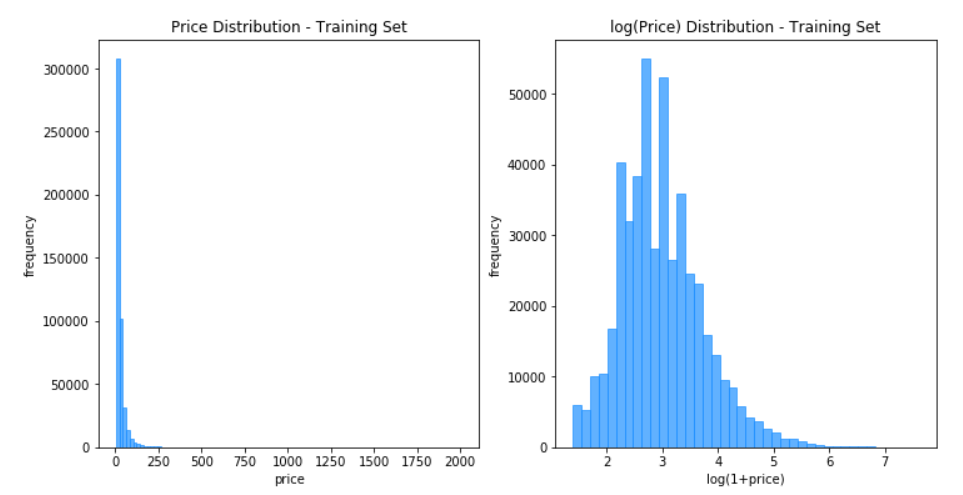
price
By looking at the data after visualization we know why we have to do log1p on price to make the distribution of price better.

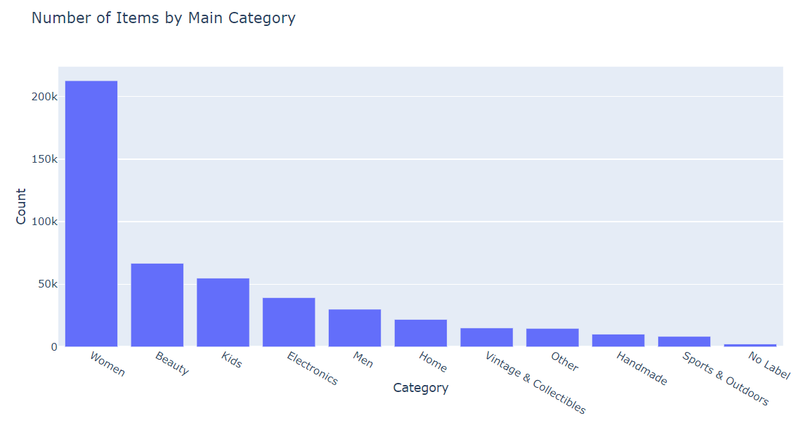
category_name
Try to split the property into various subclasses and view the corresponding data.

item_description

Try different attributes combination

simply combine the attributes together in the sample code for text analysis, i.e. name + item_condition_id + category_name + brand_name + shipping + item_description. (6 inputs)
try name, item_condition_id, shipping,category_name + item_description, brand_name. (5 inputs)
try name, item_condition_id, shipping, category_name + brand_name + item_description. (4 inputs)
try name, item_condition_id, shipping, name + category_name + brand_name + item_description. (4 inputs)

The results for the four combinations as input are very similar, except that combination 1 MSLE is around 0.4, combinations 2 and 3 are around 0.21, and combination 4 eventually runs to around 0.17. Combination 4 actually increases the weight of name to make the final result better.

Final source code and experimental results

Data preprocessing

# data preprocessing
# There are 8 attributes, remove price, train_id will have no influence on the result.
def data_preprocess(df):
    df['name'] = df['name'].fillna('') + ' ' + df['brand_name'].fillna('')
    df['text'] = (df['item_description'].fillna('') + ' ' + df['name'] + ' ' + df['category_name'].fillna(''))
    return df[['name', 'text', 'shipping', 'item_condition_id']]

Model Construction

def fit_predict(xs, y_train):
    X_train, X_test = xs
    # Configure the operation method of tf.Session, such as gpu operation or cpu operation
    config = tf.ConfigProto(
        # Set the number of threads for multiple operations in parallel
        intra_op_parallelism_threads=1, use_per_session_threads=1, inter_op_parallelism_threads=1)
    # Session provides the environment for Operation execution and Tensor evaluation.
    with tf.Session(graph=tf.Graph(), config=config) as sess, timer('fit_predict'):
        ks.backend.set_session(sess)
        model_in = ks.Input(shape=(X_train.shape[1],), dtype='float32', sparse=True)
        # ks.layers.Dense means the dimension of output
        # Dense full connected layer, equals to add one layer directly.
        # activation is the activation function.
        out = ks.layers.Dense(192, activation='relu')(model_in)
        out = ks.layers.Dense(64, activation='relu')(out)
        out = ks.layers.Dense(64, activation='relu')(out)
        out = ks.layers.Dense(1)(out)
        model = ks.Model(model_in, out)
        model.compile(loss='mean_squared_error', optimizer=ks.optimizers.Adam(lr=3e-3))
        for i in range(3):
            with timer(f'epoch {i + 1}'):
                model.fit(x=X_train, y=y_train, batch_size=2 ** (11 + i), epochs=1, verbose=0)
        return model.predict(X_test)[:, 0]

Model training and prediction

def main():
    vectorizer = make_union(# Assemble all transformers into a FeatureUnion. n_jobs means it can be done simultaneously
        # FunctionTransformer implements a custom transformation with no input validation when validate=False
        # TfidfVectorizer function, consider only the words in the first max_feature bits by word frequency, token_pattern='\w+' matches at least one word
        make_pipeline(FunctionTransformer(itemgetter('name'), validate=False), TfidfVectorizer(max_features=100000, token_pattern='\w+')),
        make_pipeline(FunctionTransformer(itemgetter('text'), validate=False), TfidfVectorizer(max_features=100000, token_pattern='\w+')),
        make_pipeline(FunctionTransformer(itemgetter(['shipping', 'item_condition_id']), validate=False),
                      FunctionTransformer(to_records, validate=False), DictVectorizer()),
        n_jobs=4)
    # StandardScaler() performs data normalization. Save the parameters (mean, variance) from the training set directly using its object to transform the test set data.
    y_scaler = StandardScaler()
    # The with statement is used when accessing resources to ensure that the necessary "cleanup" operations are performed to release resources regardless of exceptions during use, such as automatic closure of files after use, automatic acquisition and release of locks in threads, etc.
    with timer('process train'):
        train = pd.read_csv('train.csv', sep='\t')
        test = pd.read_csv('test.csv', sep='\t')
        # remove 'price'
        train = train[train['price'] > 0].reset_index(drop=True)
        # normalization of price
        y_train = y_scaler.fit_transform(np.log1p(train['price'].values.reshape(-1, 1)))
        X_train = vectorizer.fit_transform(data_preprocess(train)).astype(np.float32)
        print(f'X_train: {X_train.shape} of {X_train.dtype}')
    with timer('process valid'):
        X_test = vectorizer.transform(data_preprocess(test)).astype(np.float32)
    with ThreadPool(processes=4) as pool:
        Xb_train, Xb_test = [x.astype(np.bool).astype(np.float32) for x in [X_train, X_test]]
        xs = [[Xb_train, Xb_test], [X_train, X_test]] * 2
        # prediction
        y_pred = np.mean(pool.map(partial(fit_predict, y_train=y_train), xs), axis=0)
    y_pred = np.expm1(y_scaler.inverse_transform(y_pred.reshape(-1, 1))[:, 0])
    # print(type(y_pred))

    # Export prediction results to csv
    test_id = np.array(range(0, len(y_pred)))
    dataframe = pd.DataFrame({'test_id': test_id, 'price': y_pred})
    dataframe.to_csv("res.csv", index=False, sep='\t')

    # print('Valid MSLE: {:.4f}'.format(mean_squared_log_error(valid['price'], y_pred)))

The final experimental result reached 0.179.

Other optimization directions in the `MLP` model

It can be observed that in the word cloud of item_desciption, there are words such as shipping and free, which may stand for free shipping and other meanings, and there is some duplication with the shipping attribute, and using it as a feature word to train the model will cause interference.
The information contained in a single keyword may not be comprehensive, and there may be great correlation between keywords.
In the final model MLP uses a four-layer perceptron, and the number of layers of the perceptron and the input size of each layer can be further tuned.

Experience

This experiment was very difficult and I didn’t know where to start.

After carefully studying the sample code given in the course and the content of data visualization and analysis, I got a preliminary understanding of both the dataset and the method of prediction.

Since I was very unfamiliar with models such as MLP and Lightgbm, I started from the input point of view and experimented with the combination of different attributes to get the final and better results.

In the following study, we should learn and understand the model more deeply, and try to create the model independently, instead of modifying other models that have been written.